Accelerated factorized backprojection (AFBP)

FFBP and CFBP (see their examples) reduce the cost of backprojection by imaging subapertures on coarse grids and merging them recursively, paying for the speedup with interpolation error at every merge level. AFBP removes the interpolation completely by merging in the wavenumber domain:

1. Split the aperture into subapertures and backproject each one onto the same polar grid, decimated in azimuth. Unlike FFBP, the grid origin is the same same on all subapertures, a target sits at the same \((r, \theta)\) cell in every subaperture image.

2. Because the grids share an origin, each subaperture image holds a contiguous patch of the full image’s azimuth wavenumber spectrum, aliased onto the decimated grid. The full-resolution image is assembled by FFT of the subaperture images, placing each patch at its true position in the full spectrum, and inverse FFT. No interpolation needed.

The fusion is a single level (no recursion), so the backprojection cost drops by the number of subapertures while the fusion costs a few FFTs. The output matches direct backprojection including pixel phase far more accurately than the recursive interpolating merges, which makes AFBP attractive on short apertures, either standalone or as the base layer of FFBP (ffbp(..., afbp_nsub=...)).

The library exposes this as a single call, torchbp.ops.afbp. In this notebook the algorithm is built by hand from backprojection_polar_2d and a few lines of torch to demonstrate how it works.

Reference: L. Zhang, H.-l. Li, Z.-j. Qiao and Z.-w. Xu, “A Fast BP Algorithm With Wavenumber Spectrum Fusion for High-Resolution Spotlight SAR Imaging,” IEEE Geoscience and Remote Sensing Letters, vol. 11, no. 9, pp. 1460-1464, Sept. 2014.

import math
import torch
import numpy as np
import matplotlib.pyplot as plt
from numpy import hamming

import torchbp
from torchbp.ops import backprojection_polar_2d

device = "cuda" if torch.cuda.is_available() else "cpu"
print("Device:", device)

Device: cpu

Scene and radar parameters

A single point target imaged on a heavily oversampled polar grid zoomed around the target, same setup as the FFBP example. The platform track is along y (cross-range), boresight along x, theta is the sine of the azimuth angle.

fc = 6e9          # RF center frequency (Hz)
bw = 200e6        # RF bandwidth (Hz), positive for rising sweep
tsweep = 100e-6   # Sweep length (s)
fs = 2e6          # Sampling frequency (Hz)
nsweeps = 512     # Number of pulses in the aperture
oversample = 2    # Range FFT oversampling (reduces interpolation error)
nsamples = int(fs * tsweep)

# Heavily oversampled polar grid, zoomed on the target. theta is sin(angle).
nr, ntheta = 256, 512
grid = {"r": (96.0, 104.0), "theta": (-0.06, 0.06), "nr": nr, "ntheta": ntheta}

# Single point target at 100 m, broadside.
target_pos = torch.tensor([[100.0, 0.0, 0.0]], dtype=torch.float32, device=device)
target_rcs = torch.ones((1, 1), dtype=torch.float32, device=device)

# Straight platform track along y at 50 m height. Element spacing = lambda/4.
pos = torch.zeros((nsweeps, 3), dtype=torch.float32, device=device)
pos[:, 1] = torch.linspace(-nsweeps / 2, nsweeps / 2, nsweeps, device=device) * 0.25 * 3e8 / fc
pos[:, 2] = 50.0

Simulate and range-compress the data

Identical to the backprojection example. Generate raw data, apply a range window, and FFT to range-compress. data_fmod shifts the data spectrum to DC and alias_fmod centers the image spectrum, both reduce interpolation error inside backprojection and must be passed consistently everywhere. The wavenumber fusion accounts for both.

raw = torchbp.util.generate_fmcw_data(target_pos, target_rcs, pos, fc, bw, tsweep, fs)
w = torch.tensor(hamming(raw.shape[-1])[None, :], dtype=torch.float32, device=device)
data = torch.fft.ifft(raw * w, dim=-1, n=nsamples * oversample)

data_fmod = -math.pi * (1 - (oversample - 1) / oversample)
data = data * torch.exp(1j * data_fmod * torch.arange(data.shape[-1], device=device))[None, :]

r_res = 3e8 / (2 * abs(bw) * oversample)           # range bin size in the data
dr = (grid["r"][1] - grid["r"][0]) / grid["nr"]    # range bin size in the image
im_margin = oversample * r_res / dr - 1
alias_fmod = -math.pi * (1 - im_margin / (1 + im_margin))
print(f"r_res={r_res:.3f} m, image dr={dr:.3f} m, data_fmod={data_fmod:.3f}, alias_fmod={alias_fmod:.3f}")

r_res=0.375 m, image dr=0.031 m, data_fmod=-1.571, alias_fmod=-0.131

A small helper to display a polar image in dB.

extent = [*grid["r"], *grid["theta"]]

def show_polar(img, title, ax=None, dyn=30, ref_max=None):
    img = img.detach().cpu()
    db = 20 * torch.log10(torch.abs(img) + 1e-12)
    m = db.max() if ref_max is None else ref_max
    if ax is None:
        _, ax = plt.subplots()
    im = ax.imshow(db.numpy().T, origin="lower", vmin=m - dyn, vmax=m,
                   extent=extent, aspect="auto")
    ax.set_title(title)
    ax.set_xlabel("Range (m)")
    ax.set_ylabel("Angle (sin)")
    return m

def relerr(a, b):
    return (torch.linalg.norm(a - b) / torch.linalg.norm(a)).item()

Reference: Direct backprojection

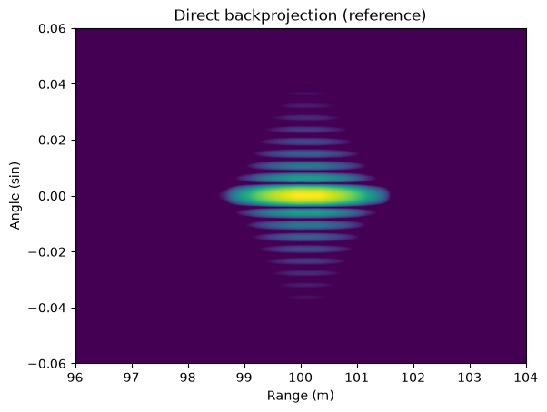
dealias=True removes the range carrier \(\exp(j \pi k_\text{eff} d(r))\), \(d(r) = \sqrt{r^2 + z_0^2}\), from the image. This is required for AFBP subapertures to get a compact spectrum (see SAR image interpolation example).

img_bp = backprojection_polar_2d(
    data, grid, fc, r_res, pos, dealias=True, data_fmod=data_fmod, alias_fmod=alias_fmod
).squeeze()

m = show_polar(img_bp, "Direct backprojection (reference)")

Step 1: Backproject the subapertures on the shared coarse grid

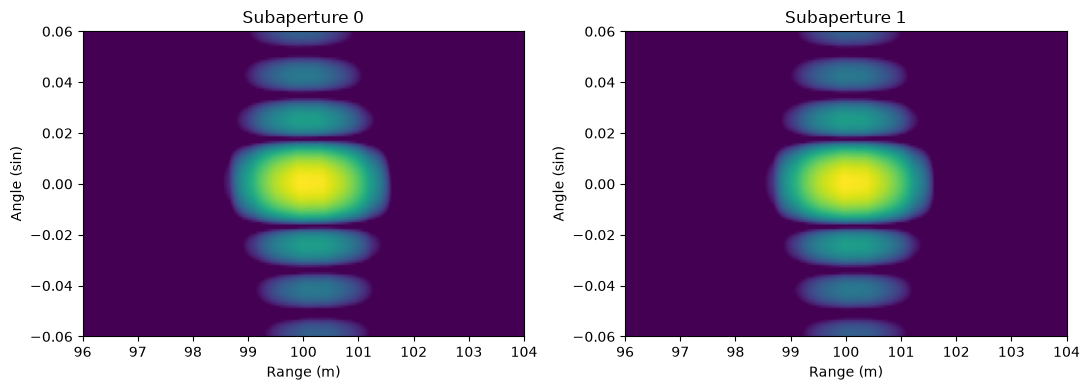
Split the aperture into NSUB parts and backproject each onto the global grid with ntheta / NSUB azimuth samples. This is the key difference to FFBP: the positions are not re-centered per subaperture and every subaperture uses the same grid extents, so all images are in the same coordinate frame. Each subaperture has 1 / NSUB of the pulses and 1 / NSUB of the pixels, and there are NSUB of them. The total backprojection cost is 1 / NSUB of the direct one.

The subaperture images look identical to FFBP’s at first glance, coarse azimuth resolution, full range resolution, but the target sits at the same cell in each and, each image keeps the azimuth carrier of its off-center aperture position.

NSUB = 4
n_c = ntheta // NSUB
grid_c = dict(grid, ntheta=n_c)
n = nsweeps // NSUB

imgs, x_u = [], []
for u in range(NSUB):
    sl = slice(u * n, (u + 1) * n)
    img_u = backprojection_polar_2d(
        data[sl], grid_c, fc, r_res, pos[sl],
        dealias=True, data_fmod=data_fmod, alias_fmod=alias_fmod,
    ).squeeze()
    imgs.append(img_u)
    x_u.append(float(pos[sl, 1].mean()))  # along-track subaperture centers
imgs = torch.stack(imgs)

print("subaperture image shape:", tuple(imgs.shape[1:]), "(full grid is", (nr, ntheta), ")")
print("subaperture centers x_u:", [f"{x:.2f}" for x in x_u])
fig, axs = plt.subplots(1, 2, figsize=(11, 4))
show_polar(imgs[0], "Subaperture 0", ax=axs[0])
show_polar(imgs[1], "Subaperture 1", ax=axs[1])
plt.tight_layout();

subaperture image shape: (256, 128) (full grid is (256, 512) )
subaperture centers x_u: ['-2.40', '-0.80', '0.80', '2.40']

Why the subapertures are spectrum patches

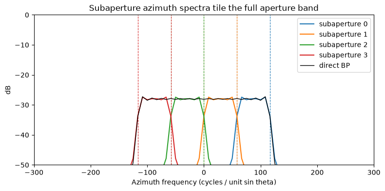
For a pixel at \((r, \alpha)\) (\(\alpha = \sin \theta\)) and a pulse at along-track position \(x\), the two-way distance is \(d = \sqrt{r^2 - 2 r \alpha x \cdot r/d_s + \dots}\) and to first order in \(x\) the dealiased image of subaperture \(u\) carries the azimuth phase

\[\exp\!\big({-j k \, x_u \, \tfrac{r}{d_s(r)} \, (\alpha - \alpha_p)}\big), \qquad d_s(r) = \sqrt{r^2 + z_0^2},\]

where \(k = 4\pi f_c / c - f_\text{mod,data} / \Delta_r\) is the effective range wavenumber of the image and \(\alpha_p\) the target angle. A linear phase in \(\alpha\) is a shifted spectrum: subaperture \(u\) occupies the azimuth frequency band centered at \(-k\, x_u\, r/d_s / (2\pi)\) cycles per unit \(\alpha\), with width set by the subaperture length. The factor \(r / d_s\) is the ground-to-slant range ratio: the classical algorithm assumes a slant-plane image where it is 1, on the torchbp ground-range grid it scales the patch positions (here evaluated at the swath center; the library op follows its range variation with range blocks).

The plot shows the azimuth spectrum of each subaperture image formed on the full grid: four flat patches that tile the full aperture band (dashed lines are the predicted patch edges). The coarse ntheta / NSUB grid of step 1 samples each patch critically, that is why one subaperture needs only 1 / NSUB of the azimuth samples.

C0 = 299792458.0
krc = 4 * math.pi * fc / C0 - data_fmod / r_res  # effective range wavenumber (rad/m)
z0 = float(pos[:, 2].mean())
r_mid = 0.5 * (grid["r"][0] + grid["r"][1])
fac = r_mid / math.sqrt(r_mid**2 + z0**2)        # ground-to-slant factor
dalpha = (grid["theta"][1] - grid["theta"][0]) / ntheta
L_sub = float(pos[n, 1] - pos[0, 1])             # subaperture length

nu = np.fft.fftshift(np.fft.fftfreq(ntheta, d=dalpha))
plt.figure(figsize=(9, 4))
for u in range(NSUB):
    sl = slice(u * n, (u + 1) * n)
    img_f = backprojection_polar_2d(
        data[sl], grid, fc, r_res, pos[sl],
        dealias=True, data_fmod=data_fmod, alias_fmod=alias_fmod,
    ).squeeze()
    s = np.abs(np.fft.fftshift(np.fft.fft(img_f.cpu().numpy(), axis=-1), axes=-1)).mean(0)
    line, = plt.plot(nu, 20 * np.log10(s + 1e-9), label=f"subaperture {u}")
    center = -krc * x_u[u] * fac / (2 * math.pi)
    hw = krc * L_sub * fac / (4 * math.pi)
    plt.axvline(center - hw, color=line.get_color(), ls="--", lw=0.8)
    plt.axvline(center + hw, color=line.get_color(), ls="--", lw=0.8)
s = np.abs(np.fft.fftshift(np.fft.fft(img_bp.cpu().numpy(), axis=-1), axes=-1)).mean(0)
plt.plot(nu, 20 * np.log10(s + 1e-9), "k", lw=1, label="direct BP")
plt.xlim(-300, 300); plt.ylim(-50, 0)
plt.xlabel("Azimuth frequency (cycles / unit sin theta)")
plt.ylabel("dB")
plt.title("Subaperture azimuth spectra tile the full aperture band")
plt.legend();

Step 2: Wavenumber fusion

On the coarse grid each patch is aliased, but nothing is lost: the coarse grid samples every NSUB-th point of the fine grid, so a coarse spectrum bin is the sum of the fine spectrum aliases, \(S_c[k] = \frac{1}{N_\text{sub}} \sum_j S_f[k + j\, n_c]\). Inside the patch the other aliases are just the patch’s own leakage tails, so the fine bin \(m\) is recovered with plain indexing:

\[S_f[m] \approx N_\text{sub} \; S_c[m \bmod n_c].\]

There is no explicit circular shift and no interpolation, the patch placement is the index arithmetic. Two refinements make it accurate:

• Trapezoidal placement: the patch center is proportional to the range wavenumber \(k_r\), not just its center value, so the assembly runs per range-wavenumber row (range FFT first, x_eq below is the along-track position owning each row/bin).

• Overlapping regions summed: a discrete patch has leakage tails past its rect edges. Assigning each fine bin to exactly one subaperture (hard tiling) truncates the tails at every seam, which costs surprisingly much (~-20 dB). Instead every subaperture reconstructs a full coarse band centered on its own patch and the overlapping regions of adjacent subapertures are summed, near a seam the true spectrum really is the sum of both patches edge transitions.

Note that linear track and \((r, \sin \theta)\) grid assumptions are used here. If either assumption doesn’t hold then the subaperture spectrum relationship is more complicated.

Everything is exact bookkeeping of the FFT bin frequencies: nu_c is where the data_fmod/alias_fmod modulations put the range spectrum center.

N = ntheta
Sa = torch.fft.fft(imgs, dim=-1)   # azimuth FFT -> aliased patches
S = torch.fft.fft(Sa, dim=-2)      # range FFT -> range wavenumber rows

# Range wavenumber of every row, unwrapped around the modulation-shifted center.
nu_c = alias_fmod / (2 * dr) - data_fmod / (2 * r_res)
fr = torch.fft.fftfreq(nr, d=dr, dtype=torch.float64, device=device)
half = 1 / (2 * dr)
kr = krc + 2 * math.pi * (torch.remainder(fr - nu_c + half, 2 * half) - half)

# Along-track position owning each (range wavenumber row, fine azimuth bin).
nua = torch.fft.fftfreq(N, d=dalpha, dtype=torch.float64, device=device)
x_eq = -2 * math.pi * nua[None, :] / (kr[:, None] * fac)
# Half width of one coarse band in the same units.
x_half = math.pi * n_c / (N * dalpha) / (kr * fac)

cols = torch.arange(N, device=device) % n_c
fine = S.new_zeros((nr, N))
for u in range(NSUB):
    mask = (x_eq - x_u[u]).abs() <= x_half[:, None].abs()
    fine += S[u, :, cols] * mask
fine *= NSUB

img_afbp = torch.fft.ifft(torch.fft.ifft(fine, dim=-2), dim=-1)

fig, axs = plt.subplots(1, 2, figsize=(11, 4))
show_polar(img_bp, "Direct backprojection", ax=axs[0], ref_max=m)
show_polar(img_afbp, f"AFBP, {NSUB} subapertures (manual)", ax=axs[1], ref_max=m)
plt.tight_layout();

print(f"relative error vs direct BP: {relerr(img_bp, img_afbp):.4f}")

relative error vs direct BP: 0.0052

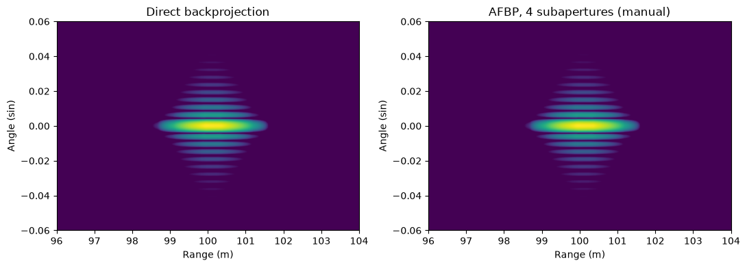
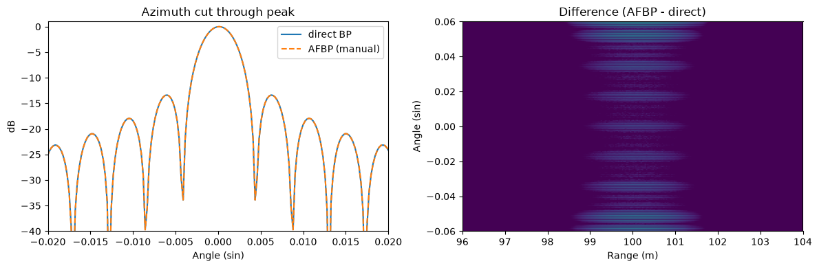
The fused image matches the reference. The azimuth cut through the peak overlays the direct result and the error floor sits far below the FFBP interpolation error on the same scene.

pk = np.unravel_index(torch.abs(img_bp).cpu().argmax(), img_bp.shape)
theta_axis = np.linspace(grid["theta"][0], grid["theta"][1], ntheta)
cut_bp = 20 * torch.log10(torch.abs(img_bp[pk[0]]).cpu() + 1e-12)
cut_af = 20 * torch.log10(torch.abs(img_afbp[pk[0]]).cpu() + 1e-12)

fig, axs = plt.subplots(1, 2, figsize=(12, 4))
axs[0].plot(theta_axis, cut_bp - cut_bp.max(), label="direct BP")
axs[0].plot(theta_axis, cut_af - cut_bp.max(), "--", label="AFBP (manual)")
axs[0].set_xlim(-0.02, 0.02); axs[0].set_ylim(-40, 1)
axs[0].set_xlabel("Angle (sin)"); axs[0].set_ylabel("dB")
axs[0].set_title("Azimuth cut through peak"); axs[0].legend()
show_polar(img_bp - img_afbp, "Difference (AFBP - direct)", ax=axs[1], ref_max=m, dyn=80)
plt.tight_layout();

/tmp/ipykernel_2935/1064639533.py:1: DeprecationWarning: __array__ implementation doesn't accept a copy keyword, so passing copy=False failed. __array__ must implement 'dtype' and 'copy' keyword arguments. To learn more, see the migration guide https://numpy.org/devdocs/numpy_2_0_migration_guide.html#adapting-to-changes-in-the-copy-keyword
  pk = np.unravel_index(torch.abs(img_bp).cpu().argmax(), img_bp.shape)

Library op torchbp.ops.afbp

Everything above is what torchbp.ops.afbp does internally, plus:

• a theta guard band (guard_theta): the subaperture images treat theta as circular, so a target near the grid edge wraps around with a broadband spectral skirt. The guard moves the wrap point outside the scene and is cropped from the output

• range blocks that follow the ground-to-slant factor \(r / d_s(r)\) over a wide swath instead of using one swath-center value

• uneven pulse/theta splits, batched subaperture backprojection, and validity warnings (patch fit on the decimated grid, quadratic phase error bound)

img_lib4 = torchbp.ops.afbp(data, grid, fc, r_res, pos, nsub=4, dealias=True,
                            data_fmod=data_fmod, alias_fmod=alias_fmod)
img_lib8 = torchbp.ops.afbp(data, grid, fc, r_res, pos, nsub=8, dealias=True,
                            data_fmod=data_fmod, alias_fmod=alias_fmod)

print(f"afbp nsub=4 vs direct BP: {relerr(img_bp, img_lib4):.4f}")
print(f"afbp nsub=8 vs direct BP: {relerr(img_bp, img_lib8):.4f}")

afbp nsub=4 vs direct BP: 0.0003
afbp nsub=8 vs direct BP: 0.0003

AFBP as the FFBP base layer

The single-level fusion assumes a straight track and a quadratic-phase bound \(\alpha_\text{max} \, l \le r_0 / 4\) per subaperture, so it cannot replace FFBP for very long, curved apertures. There it can still speed up the base level, where the subapertures are short and the direct backprojections dominate the cost: ffbp(..., afbp_nsub=N) computes each base-level image with AFBP, cutting the base cost roughly N times.

Note what this does and does not buy. As a drop-in addition it does not improve accuracy: the FFBP merge interpolation error dominates, and the AFBP base only adds a much smaller error on top (compare the first two lines below). The benefit is the cost trade, because the base level gets N times cheaper, an interpolating merge stage can be dropped at roughly constant total cost. stages=1, afbp_nsub=4 has about the same base-level cost as stages=3 but only one interpolating merge instead of three, so it runs at the deep-recursion speed with the shallow-recursion accuracy (last line).

for stages, ans in [(2, 1), (2, 4), (1, 1), (1, 4)]:
    img = torchbp.ops.ffbp(data, grid, fc, r_res, pos, stages=stages, dealias=True,
                           data_fmod=data_fmod, alias_fmod=alias_fmod, afbp_nsub=ans)
    print(f"ffbp stages={stages} afbp_nsub={ans} vs direct BP: {relerr(img_bp, img):.4f}")

ffbp stages=2 afbp_nsub=1 vs direct BP: 0.0316
ffbp stages=2 afbp_nsub=4 vs direct BP: 0.0316
ffbp stages=1 afbp_nsub=1 vs direct BP: 0.0089
ffbp stages=1 afbp_nsub=4 vs direct BP: 0.0089

/home/runner/work/torchbp/torchbp/torchbp/ops/ffbp.py:554: UserWarning: ffbp: theta guard band capped at 22 bins (46 needed for full interpolation support at the near range edge). Edge accuracy at near range may be reduced; increase guard_max_ratio (more memory) if it matters.
  warn(f"ffbp: theta guard band capped at {guard_shortfall[2]} bins "

Benefit and downside

AFBP gives the subaperture speedup of one factorization level with no interpolation error: the fusion is exact up to the discrete patch-edge effects handled by the overlap-sum and the guard band, and in practice sits one to two orders of magnitude below the FFBP merge error while being faster on short apertures. It also preserves pixel phase, so interferometric or autofocus processing downstream is unaffected, and the whole pipeline is differentiable with respect to the data.

The downsides are the assumptions the spectrum placement is built on: an approximately straight track along y, patch positions linear in \(\alpha\) (the quadratic phase bound \(\alpha_\text{max} l \le r_0/4\)), and an azimuth grid fine enough that one subaperture patch fits the decimated band (\(\Delta\alpha \le \lambda_\text{min} / (2 L / N_\text{sub})\), the op warns when violated). Wide total angles, long curved tracks, or strong altitude variation are handled by FFBP; there ffbp(..., afbp_nsub=N) trades interpolating merge stages for the interpolation-free fusion, keeping the deep-recursion speed with fewer merge stages worth of error.