Generalized phase gradient autofocus (GPGA)

In real Synthetic Aperture Radar (SAR) acquisitions the platform never follows its nominal trajectory exactly. Even small uncompensated motion errors translate into phase errors across the synthetic aperture, which blur and defocus the backprojected image.

Generalized phase gradient autofocus (GPGA) with trajectory deviation estimation estimates these errors directly from the data. The image is split into several subimages spread across range and azimuth. The slant-range error to each subimage is estimated from its phase history, and a 3D position error of the platform is then solved from the collection of slant-range errors.

This example simulates a moving FMCW radar with a random motion error, images it with an backprojection, and then recovers the trajectory using torchbp.autofocus.gpga_bp_polar_tde.

import torch
import numpy as np
import torchbp
import matplotlib.pyplot as plt
from numpy import hamming
from torchbp.util import detrend

torch.manual_seed(125);

Use CUDA if available.

if torch.cuda.is_available():
    device = "cuda"
else:
    device = "cpu"
print("Device:", device)

Device: cpu

Radar and acquisition geometry

We model a small FMCW radar flown along the \(y\) axis at 20 m altitude, looking in the \(+x\) direction. The platform records nsweeps measurements that together form the synthetic aperture.

ntheta = 512    # Azimuth points in the image
nsweeps = 512   # Number of measurements (aperture positions)
fc = 6e9        # RF center frequency (Hz)
bw = 300e6      # RF bandwidth (Hz)
tsweep = 200e-6 # Sweep length (s)
fs = 3e6        # Sampling frequency (Hz)
nsamples = int(fs * tsweep)  # Time-domain samples per sweep

wl = 3e8 / fc                # Wavelength (m)
range_res = 3e8 / (2 * bw)   # Range resolution (m)

# Imaging grid. Azimuth angle "theta" is sin of radians.
nr = 2 * int(1 + (70 - 30) / range_res)
grid_polar = {"r": (30, 70), "theta": (-0.7, 0.7), "nr": nr, "ntheta": ntheta}

Targets

The scene is a 5x5 grid of point targets.

targets = []
for x in np.linspace(35, 65, 5):
    for y in np.linspace(-20, 20, 5):
        targets.append([x, y, 0])
target_pos = torch.tensor(targets, dtype=torch.float32, device=device)
target_rcs = torch.ones(target_pos.shape[0], dtype=torch.float32, device=device)

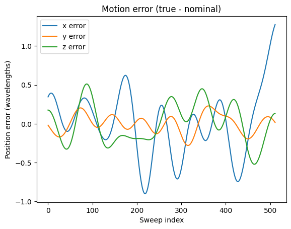
Nominal trajectory and motion error

pos is the true trajectory the platform actually flew and pos_error is the ideal trajectory: a straight line along \(y\) at a fixed altitude. The difference between them is a smooth, band-limited random motion error added to all three axes. It’s generated by low-pass filtering white noise in the frequency domain.

Linear trend is removed since it can’t be solved since it only shifts the image.

The autofocus algorithm only gets to see the nominal pos_error and its job is to recover pos.

pos = torch.zeros([nsweeps, 3], dtype=torch.float32, device=device)
pos[:, 1] = torch.linspace(-nsweeps / 2, nsweeps / 2, nsweeps) * 0.25 * wl
pos[:, 2] = 20

# Nominal trajectory without motion error
pos_error = pos.clone()

window_width = nsweeps // 32  # Low-pass cutoff for the error spectrum
error_scale = 10

def bandlimited_error(scale):
    "Smooth band-limited random error in units of wavelength * scale"
    r = scale * torch.rand(nsweeps, device=device) * wl
    fdata = torch.fft.fft(r)
    fdata[window_width // 2:-window_width // 2] = 0
    return torch.fft.ifft(fdata).real

# Range (x), Along-track (y) and vertical (z) motion errors.
pos[:, 0] = detrend(bandlimited_error(error_scale))
pos[:, 0] -= torch.mean(pos[:, 0])

ey = bandlimited_error(0.25 * error_scale)
ey -= torch.mean(ey)
pos[:, 1] += detrend(ey)

ez = bandlimited_error(0.5 * error_scale)
ez -= torch.mean(ez)
pos[:, 2] += detrend(ez)

print("Track length:", (pos[-1, 1] - pos[0, 1]).item(), "m")

Track length: 6.401793003082275 m

plt.figure()
plt.title("Motion error (true - nominal)")
plt.plot((pos[:, 0] - pos_error[:, 0]).cpu().numpy() / wl, label="x error")
plt.plot((pos[:, 1] - pos_error[:, 1]).cpu().numpy() / wl, label="y error")
plt.plot((pos[:, 2] - pos_error[:, 2]).cpu().numpy() / wl, label="z error")
plt.xlabel("Sweep index")
plt.ylabel("Position error (wavelengths)")
plt.legend(loc="best");

Generate raw radar data

generate_fmcw_data simulates the range-compressed FMCW echoes seen along the true trajectory pos. We apply a Hamming window in range and inverse FFT with oversampling to reduce interpolation errors during backprojection.

# Oversampling input data decreases interpolation errors.
oversample = 3

with torch.no_grad():
    data = torchbp.util.generate_fmcw_data(
        target_pos, target_rcs, pos, fc, bw, tsweep, fs, rvp=False)
    # Apply windowing function in range direction.
    w = torch.tensor(hamming(data.shape[-1])[None, :],
                     dtype=torch.float32, device=device)
    data = torch.fft.ifft(data * w, dim=-1, n=nsamples * oversample)

r_res = 3e8 / (2 * bw * oversample)  # Range bin size in the input data

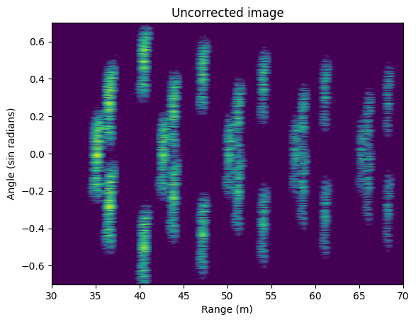
Uncorrected image

Backprojecting with the nominal trajectory pos_error has motion errors, so the point targets are defocused.

img = torchbp.ops.backprojection_polar_2d(data, grid_polar, fc, r_res, pos_error)
img = img.squeeze()  # Remove singular batch dimension

img_db = 20 * torch.log10(torch.abs(img)).detach()
m = torch.max(img_db)
extent = [*grid_polar["r"], *grid_polar["theta"]]

plt.figure()
plt.title("Uncorrected image")
plt.imshow(img_db.cpu().numpy().T, origin="lower", vmin=m - 30, vmax=m,
           extent=extent, aspect="auto")
plt.xlabel("Range (m)")
plt.ylabel("Angle (sin radians)");

Run GPGA autofocus

gpga_bp_polar_tde divides the image into range_divisions x azimuth_divisions subimages, estimates the slant-range error to each, and solves for the 3D platform position. estimate_z=True recovers the cross-track \(z\) error as well, which is possible here because the look angle variation is large.

It returns the refocused image and the recovered trajectory pos_new.

img_pga, pos_new = torchbp.autofocus.gpga_bp_polar_tde(
    img, data, pos_error, fc, r_res, grid_polar,
    range_divisions=3, azimuth_divisions=3, estimate_z=True)

rms = lambda a, b: torch.sqrt(torch.mean(torch.square(a - b))).item()
print("RMS error total:", 1e3*rms(pos_new, pos), "mm")
print("RMS error X:", 1e3*rms(pos_new[:, 0], pos[:, 0]), "mm")
print("RMS error Y:", 1e3*rms(pos_new[:, 1], pos[:, 1]), "mm")
print("RMS error Z:", 1e3*rms(pos_new[:, 2], pos[:, 2]), "mm")

RMS error total: 0.38229257916100323 mm
RMS error X: 0.23626783513464034 mm
RMS error Y: 0.3550225810613483 mm
RMS error Z: 0.5065366276539862 mm

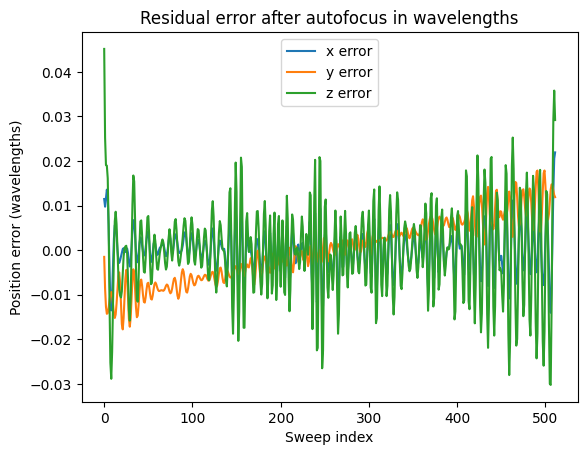
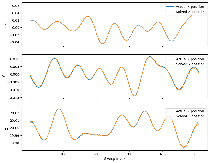
Recovered trajectory

The residual error between the recovered trajectory and the true one should be small if everything went correctly.

pos_new_np = pos_new.cpu().numpy().T

plt.figure()
plt.title("Residual error after autofocus in wavelengths")
plt.plot((pos[:, 0].cpu().numpy() - pos_new_np[0]) / wl, label="x error")
plt.plot((pos[:, 1].cpu().numpy() - pos_new_np[1]) / wl, label="y error")
plt.plot((pos[:, 2].cpu().numpy() - pos_new_np[2]) / wl, label="z error")
plt.legend(loc="best")
plt.xlabel("Sweep index")
plt.ylabel("Position error (wavelengths)");

fig, axs = plt.subplots(3, 1, figsize=(10, 8), sharex=True)

axs[0].plot(pos[:, 0].cpu().numpy(), label="Actual X position")
axs[0].plot(pos_new_np[0], label="Solved X position")
axs[0].legend(loc="upper right")
axs[0].set_ylabel("X")

# Subtract the (large) nominal track from y so the error is visible.
axs[1].plot(pos[:, 1].cpu().numpy() - pos_error[:, 1].cpu().numpy(),
            label="Actual Y position")
axs[1].plot(pos_new_np[1] - pos_error[:, 1].cpu().numpy(),
            label="Solved Y position")
axs[1].legend(loc="upper right")
axs[1].set_ylabel("Y")

axs[2].plot(pos[:, 2].cpu().numpy(), label="Actual Z position")
axs[2].plot(pos_new_np[2], label="Solved Z position")
axs[2].legend(loc="upper right")
axs[2].set_ylabel("Z")
axs[2].set_xlabel("Sweep index");

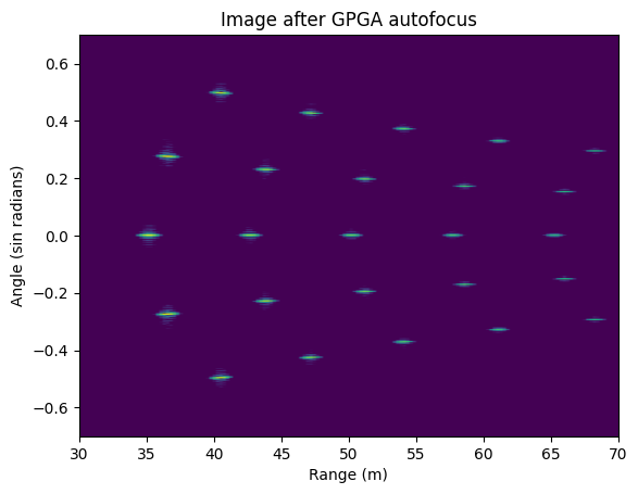
Focused image

After autofocus the point targets are well focused. The image is still in pseudo-polar coordinates.

img_pga_db = 20 * torch.log10(torch.abs(img_pga)).detach()
m = torch.max(img_pga_db)

plt.figure()
plt.title("Image after GPGA autofocus")
plt.imshow(img_pga_db.cpu().numpy().T, origin="lower", vmin=m - 30, vmax=m,
           extent=extent, aspect="auto")
plt.xlabel("Range (m)")
plt.ylabel("Angle (sin radians)");

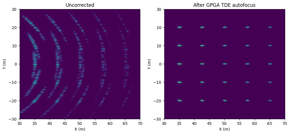
Cartesian comparison

Finally we resample both the uncorrected and the autofocused images from polar to Cartesian coordinates with polar_to_cart for a side-by-side comparison.

The correct image should look like 5x5 grid of points.

origin = torch.mean(pos_error, axis=0)
r0, r1 = grid_polar["r"]
y1 = 1.5 * (r1 - r0) / 2
grid = {"x": grid_polar["r"], "y": (-y1, y1),
        "nx": 3 * grid_polar["nr"], "ny": 3 * grid_polar["nr"]}
cart_extent = [grid["x"][0], grid["x"][1], grid["y"][0], grid["y"][1]]

def to_cart(image):
    c = torchbp.ops.polar_to_cart(torch.abs(image), origin, grid_polar, grid, fc)
    return 20 * torch.log10(torch.abs(c) + 1e-10)

img_cart = to_cart(img)
img_pga_cart = to_cart(img_pga)

fig, axs = plt.subplots(1, 2, figsize=(12, 5))
axs[0].set_title("Uncorrected")
axs[0].imshow(img_cart.cpu().numpy().T, origin="lower", vmin=m - 30, vmax=m,
              extent=cart_extent, aspect="auto")
axs[0].set_xlabel("X (m)")
axs[0].set_ylabel("Y (m)")
axs[0].grid(False)

axs[1].set_title("After GPGA TDE autofocus")
axs[1].imshow(img_pga_cart.cpu().numpy().T, origin="lower", vmin=m - 30, vmax=m,
              extent=cart_extent, aspect="auto")
axs[1].set_xlabel("X (m)")
axs[1].set_ylabel("Y (m)")
axs[1].grid(False)