SAR image interpolation

A backprojected pseudo-polar SAR image is not an absolute picture of the ground it is referenced to an origin, the mean antenna phase centre (APC) of the platform during the aperture. The range \(r\) and angle \(\theta\) of every pixel, and the carrier phase \(\exp{\left(-j 4\pi f_c r / c\right)}\) stored in it measured from the origin.

Two acquisitions flown from slightly different positions therefore land on two different polar grids. Before they can be compared, for example interferometry, they must be brought onto a common grid centred on a single origin. The brute force way is to backproject each pass again from its raw data onto the shared grid, but that is expensive.

torchbp.ops.polar_interp does the same job directly in the image domain. It resamples an already-formed polar image from its old origin/grid onto a new origin/grid, correcting both:

• the geometry, each pixel’s range and angle change when viewed from the new origin

• the carrier phase, the phase must be updated for the new range

This is the core building block of repeat-pass coregistration and of fast-factorized backprojection (FFBP), where small sub-aperture images are recuresively merged into larger more detailed image.

This example demonstrates polar_interp with synthetic data. We take one pass of raw data and form it into a polar image two ways: Directly at the new position, and by interpolating from nearby position. If polar_interp is correct the two results agree in amplitude and in phase.

import torch
import numpy as np
import torchbp
import scipy.signal as signal
import matplotlib.pyplot as plt
import time

Use CUDA if available.

if torch.cuda.is_available():
    device = "cuda"
else:
    device = "cpu"
print("Device:", device)

Device: cpu

Radar and acquisition geometry

A small FMCW radar flown along the \(y\) axis, looking towards \(+x\). We simulate two passes:

• master (pass 0), the reference geometry

• slave (pass 1), flown from a slightly different position. The slave is offset cross_track metres in \(x\), along_track metres in \(y\), and dh metres higher.

The vector between the two antenna phase centres is the baseline. Re-centring the slave image onto the master grid is exactly an origin shift by that baseline.

fc = 5.9e9          # RF center frequency (Hz)
bw = 300e6          # Sweep bandwidth (Hz)
tsweep = 200e-6     # Sweep length (s)
fs = 10e6           # Sampling frequency (Hz)
nsamples = int(fs * tsweep)   # Time-domain samples per sweep
nsweeps = 384       # Number of azimuth measurements (array elements)
wl = 3e8 / fc       # Wavelength

altitude = 50.0     # Master platform altitude (m)
cross_track = 1.0   # Slave offset across track, x (m)
along_track = 0.5   # Slave offset along track, y (m)
dh = 0.25            # Slave height above master (m)
element_spacing = 0.25 * wl   # Azimuth sampling along the track

Polar imaging grid

theta is the sine of the azimuth angle. The number of range and azimuth bins is set from the range resolution and the synthetic aperture so the grid is slightly oversampled. signal_oversample is how many grid range bins span one resolution cell, it appears again below when we centre the range spectrum for interpolation.

Higher grid oversampling factor reduces the interpolation error. If the image is aliased (oversample < 1), then interpolation can’t give the correct result as the aliased and desired sprectum overlap. This is important to get correct for interpolation to be possible.

r0, r1 = 100.0, 200.0      # Ground-range extent (m)
theta_limit = 0.7         # Azimuth half-extent (sine of angle)

res = 3e8 / (2 * bw)      # Slant-range resolution
res_interp = 2         # Grid oversampling factor
nr = int(res_interp * (r1 - r0) / res)
ntheta = int(1 + nsweeps * res_interp * (element_spacing / wl) * theta_limit / 0.25)

grid_polar = {"r": (r0, r1), "theta": (-theta_limit, theta_limit),
              "nr": nr, "ntheta": ntheta}

dr_grid = (r1 - r0) / nr
signal_oversample = res / dr_grid # How many pixels in image per resolution cell in image
print(f"nr={nr}, ntheta={ntheta}, signal_oversample={signal_oversample:.2f}")

nr=400, ntheta=538, signal_oversample=2.00

Scene

A field of random complex scatterers (speckle) on a flat ground plane. We use dense grid of scatterers so that there is at least one scatterer per resolution cell, for nice coherence plot later. This is also very difficult scene for interpolation, since the whole image is filled with scatterers.

torch.manual_seed(42)

grid_proj = {"x": (30, 210), "y": (-210, 210), "nx": 384, "ny": 384}
img = torch.randn([grid_proj["nx"], grid_proj["ny"]], dtype=torch.complex64, device=device)
dem = torch.zeros([grid_proj["nx"], grid_proj["ny"]], dtype=torch.float32, device=device)

Platform trajectories

Both passes fly straight along \(y\). The slave is rigidly shifted by the baseline. We weight the aperture with a Taylor window before computing each pass’s phase centre, matching the window applied during image formation.

y_coords = torch.linspace(-nsweeps / 2, nsweeps / 2, nsweeps) * element_spacing

# Master (pass 0)
pos0 = torch.zeros([nsweeps, 3], dtype=torch.float32, device=device)
pos0[:, 1] = y_coords.to(device)
pos0[:, 2] = altitude

# Slave (pass 1): offset by the baseline
pos1 = torch.zeros([nsweeps, 3], dtype=torch.float32, device=device)
pos1[:, 0] = cross_track
pos1[:, 1] = y_coords.to(device) + along_track
pos1[:, 2] = altitude + dh

# Aperture (azimuth) and range windows
wa = torch.tensor(signal.get_window(("taylor", 3, 30), nsweeps, fftbins=False),
                  dtype=torch.float32, device=device)
wa /= wa.mean()
wr = torch.tensor(signal.get_window(("taylor", 3, 30), nsamples, fftbins=False),
                  dtype=torch.float32, device=device)
wr /= wr.mean()

# Window-weighted antenna phase centres
apc0 = (wa[:, None] * pos0).mean(0) / wa.mean()
apc1 = (wa[:, None] * pos1).mean(0) / wa.mean()
baseline = (apc1 - apc0)
print("baseline (m):", baseline.cpu().numpy())

baseline (m): [1.0000001  0.49999997 0.25      ]

Forward projection and range compression

We simulate the slave’s raw FMCW data with projection_cart_2d_nufft, then range-compress it (windowed, oversampled inverse FFT). The data_fmod term shifts the range spectrum so that, after the oversampled transform, it sits at DC, which minimises later interpolation error. This is the same image-formation recipe used in the interferometry example.

d0 = 0
oversample = 3
n = nsamples * oversample
r_res = 3e8 / (2 * bw * oversample)
# data_fmod centers the input data spectrum decreasing interpolation errors in backprojection
data_fmod = -torch.pi * (1 - (oversample - 1) / oversample)

# Forward project the slave pass to raw FMCW data (stop-and-go NUFFT)
data = torchbp.ops.projection_cart_2d_nufft(
    img, pos1, grid_proj, fc, fs, bw / tsweep, nsamples, d0, dem,
    use_rvp=False, normalization="gamma")[0]

# Range compression: window + oversampled IFFT, then shift spectrum to DC
w = wa[:, None] * wr[None, :]
data = torch.fft.ifft(data * w, dim=-1, n=n)
data = data * torch.exp(1j * data_fmod * torch.arange(data.shape[-1], device=device))[None, :]
print("range-compressed data:", tuple(data.shape))

range-compressed data: (384, 6000)

Forming the two reference images

We backproject the same slave data twice onto the same polar grid, differing only in the origin:

• slave_own, centered on the slave’s own phase centre (apc1). This is the image we will later interpolate.

• slave_master, centered on the master’s phase centre (apc0). This is the ground truth that polar_interp must reproduce.

Backprojection is done with dealias=True. A critically sampled polar image has a range spectrum that wraps around (aliases); de-aliasing unwraps it into a clean one-sided spectrum (see torchbp.util.bp_polar_range_dealias). After de-aliasing the spectrum occupies \([0,\,2\pi/\texttt{signal\_oversample}]\) rather than being centred at DC. Interpolation is most accurate on a DC-centred signal, so we pass alias_fmod to center the spectrum at DC. The same alias_fmod is later handed to polar_interp so it knows where the spectrum sits.

alias_fmod = float(-torch.pi / signal_oversample)
print(f"alias_fmod = {alias_fmod:.4f}")

def backproject(pos_world, center_xy):
    # Center the grid under `center_xy` by shifting the platform horizontally.
    origin = torch.tensor([[center_xy[0], center_xy[1], 0.0]], device=device)
    pos_centered = pos_world - origin
    return torchbp.ops.backprojection_polar_2d(
        data, grid_polar, fc, r_res, pos_centered, d0=d0,
        dealias=True, data_fmod=data_fmod, alias_fmod=alias_fmod)[0]

t = time.time()
slave_own = backproject(pos1, apc1[:2])     # centred on slave APC
slave_master = backproject(pos1, apc0[:2])  # centred on master APC (ground truth)
print(f"Both images formed in {time.time() - t:.2f} s")

alias_fmod = -1.5708
Both images formed in 0.75 s

The two images are formed from identical data, so their magnitudes look the same. The difference lives entirely in the phase: each is referenced to a different origin.

extent = [*grid_polar["r"], *grid_polar["theta"]]
fig, axes = plt.subplots(1, 2, figsize=(11, 4))
for ax, sar, title in zip(axes, [slave_own, slave_master], ["Centred on slave APC", "Centred on master APC"]):
    db = 20 * torch.log10(torch.abs(sar) + 1e-9).cpu().numpy()
    m = db.max()
    ax.imshow(db.T, origin="lower", vmin=m - 30, vmax=m, extent=extent, aspect="auto")
    ax.set_title(title)
    ax.set_xlabel("Range (m)")
axes[0].set_ylabel("Angle (sin radians)")
plt.tight_layout();

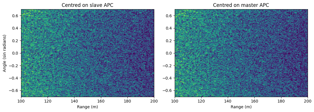
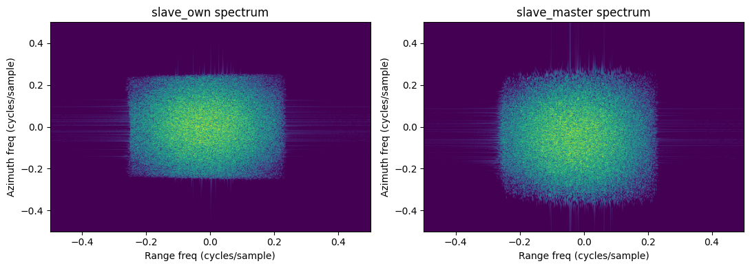
Image spectrum

For best interpolation results, the image spectrum must not be aliased and it should be centered at zero. We used dealias=True and alias_fmod to guarantee this during image formation.

Note how the spectrums of the images are slightly different due to baseline offset. slave_own positions are centered around image origin which leads to more compact spectrum than slave_master that has the baseline offset.

spec_own_db = 20*np.log10(np.abs(np.fft.fftshift(np.fft.fft2(slave_own)))).T
m = np.max(spec_own_db)

fig, axes = plt.subplots(1, 2, figsize=(11, 4))
axes[0].imshow(spec_own_db, origin="lower", aspect="auto", vmax=m, vmin=m - 40, extent=[-0.5, 0.5, -0.5, 0.5])
axes[0].set_xlabel("Range freq (cycles/sample)")
axes[0].set_ylabel("Azimuth freq (cycles/sample)")
axes[0].set_title("slave_own spectrum");

spec_master_db = 20*np.log10(np.abs(np.fft.fftshift(np.fft.fft2(slave_master)))).T

axes[1].imshow(spec_master_db, origin="lower", aspect="auto", vmax=m, vmin=m - 40, extent=[-0.5, 0.5, -0.5, 0.5])
axes[1].set_xlabel("Range freq (cycles/sample)")
axes[1].set_ylabel("Azimuth freq (cycles/sample)")
axes[1].set_title("slave_master spectrum")
plt.tight_layout();

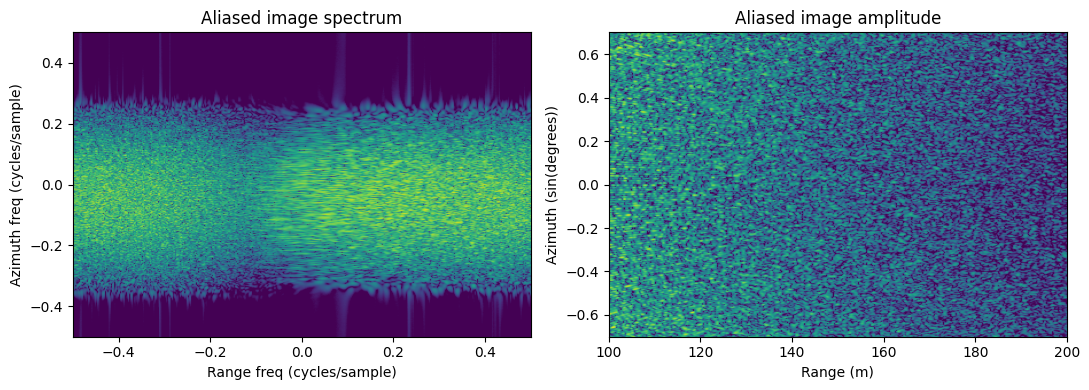
Without dealias=True and alias_fmod the spectrum of the image can be very badly aliased making it unsuitable to use for interpolation, although the amplitude of the image would be identical. torchbp.util.bp_polar_range_alias and torchbp.util.bp_polar_range_dealias can be used to alias and dealias already formed image.

It’s important for phase sensitive applications, such as interferometry, to restore the phase after interpolation using torchbp.util.bp_polar_range_alias.

# This is equivalent to if BP was called with dealias=False and alias_fmod=0
aliased = torchbp.util.bp_polar_range_alias(slave_own, apc1, fc=fc, grid_polar=grid_polar, alias_fmod=alias_fmod)

spec_aliased_db = 20*np.log10(np.abs(np.fft.fftshift(np.fft.fft2(aliased)))).T
m = np.max(spec_aliased_db)

fig, axes = plt.subplots(1, 2, figsize=(11, 4))
axes[0].imshow(spec_aliased_db, origin="lower", aspect="auto", vmax=m, vmin=m - 40, extent=[-0.5, 0.5, -0.5, 0.5])
axes[0].set_xlabel("Range freq (cycles/sample)")
axes[0].set_ylabel("Azimuth freq (cycles/sample)")
axes[0].set_title("Aliased image spectrum");

db = 20 * torch.log10(torch.abs(aliased) + 1e-9).cpu().numpy()
m = db.max()
axes[1].imshow(db.T, origin="lower", aspect="auto", vmax=m, vmin=m - 30, extent=[*grid_polar["r"], *grid_polar["theta"]])
axes[1].set_xlabel("Range (m)")
axes[1].set_ylabel("Azimuth (sin(degrees))")
axes[1].set_title("Aliased image amplitude")
plt.tight_layout();

Why re-centering is needed

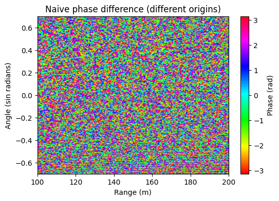
If we naively treat slave_own as if it were already on the master grid and take the phase difference against slave_master, we just get random noise. The two images disagree by the geometric phase of the baseline and the same pixel locations between to images don’t corresponds to the same location in the scene. Overlaying them directly is meaningless.

naive = torch.angle(slave_own * slave_master.conj()).cpu().numpy()
plt.figure(figsize=(6, 4))
plt.imshow(naive.T, origin="lower", cmap="hsv", extent=extent, aspect="auto")
plt.colorbar(label="Phase (rad)")
plt.xlabel("Range (m)")
plt.ylabel("Angle (sin radians)")
plt.title("Naive phase difference (different origins)")

phase_std = torch.angle(slave_own * slave_master.conj())
print(f"Phase std {torch.std(phase_std).item():.2f} rad")

Phase std 1.82 rad

Re-centering with polar_interp

Now interpolate slave_own onto the master centre. We work in the master’s centered coordinate frame:

• origin_old is where the slave image is currently referenced, the slave phase centre, which sits at baseline in the master frame. Its \(z\) is the slave’s own acquisition height.

• origin_new is the target centre, the master grid origin at horizontal \((0, 0)\), keeping the slave’s acquisition height.

polar_interp shifts every pixel from origin_old to origin_new, resampling the geometry and updating the carrier phase using fc. We use Lanczos resampling and pass the alias_fmod used during backprojection.

origin_old = torch.tensor([baseline[0].item(), baseline[1].item(), apc1[2].item()], device=device)
origin_new = torch.tensor([0.0, 0.0, apc1[2].item()], device=device)

t = time.time()
slave_interp = torchbp.ops.polar_interp(
    slave_own, origin_old=origin_old, origin_new=origin_new,
    grid_polar=grid_polar, fc=fc, rotation=0,
    grid_polar_new=grid_polar, method=("lanczos", 8),
    alias_fmod=alias_fmod)
# polar_interp may return extra batch dim; squeeze to 2D
slave_interp = slave_interp.squeeze()
print(f"polar_interp in {time.time() - t:.3f} s")

polar_interp in 0.051 s

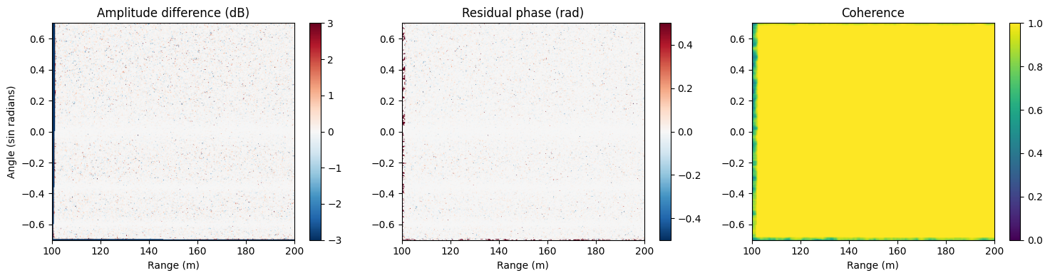
Comparison against ground truth

The interpolated image should now match the directly-backprojected slave_master. It won’t be exactly similar, since there will be some interpolation error, but it should be close. We mask off the borders (where the interpolation kernel runs out of support) and look at three things:

• amplitude ratio, should be ~1

• residual phase, \(\angle(\,s_\text{interp}\, s_\text{master}^{*})\), should be ~0

• coherence, should be ~1

The main source of error in this case is the aliasing during initial backprojection. Linear interpolation of the input data is used, which causes slight spreading of the spectrum which aliases during interpolation. However, this error is not very large and can be ignored.

mask = (torch.abs(slave_interp) > 0) & (torch.abs(slave_master) > 0)
b = 20
mask[:b, :] = False; mask[-b:, :] = False
mask[:, :b] = False; mask[:, -b:] = False

phase_res = torch.angle(slave_interp * slave_master.conj())
amp_ratio = torch.abs(slave_interp) / (torch.abs(slave_master) + 1e-10)
coh = torchbp.ops.coherence.coherence_2d(slave_interp, slave_master, (5, 5)).squeeze()

print(f"residual phase : mean {phase_res[mask].mean():+.4f}  std {phase_res[mask].std():.4f} rad")
print(f"amplitude ratio: mean {amp_ratio[mask].mean():.4f}  std {amp_ratio[mask].std():.4f}")
print(f"coherence      : mean {coh[mask].mean():.4f}")

residual phase : mean +0.0000  std 0.0361 rad
amplitude ratio: mean 1.0010  std 0.0856
coherence      : mean 0.9999

fig, axes = plt.subplots(1, 3, figsize=(15, 4))

db_m = 20 * torch.log10(torch.abs(slave_master) + 1e-9)
db_i = 20 * torch.log10(torch.abs(slave_interp) + 1e-9)
im0 = axes[0].imshow((db_i - db_m).cpu().numpy().T, origin="lower", cmap="RdBu_r",
                     vmin=-3, vmax=3, extent=extent, aspect="auto")
axes[0].set_title("Amplitude difference (dB)")
plt.colorbar(im0, ax=axes[0])

im1 = axes[1].imshow(phase_res.cpu().numpy().T, origin="lower", cmap="RdBu_r",
                     vmin=-0.5, vmax=0.5, extent=extent, aspect="auto")
axes[1].set_title("Residual phase (rad)")
plt.colorbar(im1, ax=axes[1])

im2 = axes[2].imshow(coh.cpu().numpy().T, origin="lower", vmin=0, vmax=1,
                     extent=extent, aspect="auto")
axes[2].set_title("Coherence")
plt.colorbar(im2, ax=axes[2])

for ax in axes:
    ax.set_xlabel("Range (m)")
axes[0].set_ylabel("Angle (sin radians)")
plt.tight_layout();

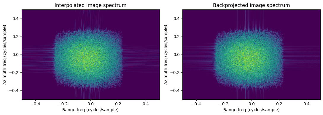
Spectrum of the interpolated image

spec_interp_db = 20*np.log10(np.abs(np.fft.fftshift(np.fft.fft2(slave_interp)))).T
m = np.max(spec_interp_db)

fig, axes = plt.subplots(1, 2, figsize=(11, 4))
axes[0].imshow(spec_interp_db, origin="lower", aspect="auto", vmax=m, vmin=m - 40, extent=[-0.5, 0.5, -0.5, 0.5])
axes[0].set_xlabel("Range freq (cycles/sample)")
axes[0].set_ylabel("Azimuth freq (cycles/sample)")
axes[0].set_title("Interpolated image spectrum");

axes[1].imshow(spec_master_db, origin="lower", aspect="auto", vmax=m, vmin=m - 40, extent=[-0.5, 0.5, -0.5, 0.5])
axes[1].set_xlabel("Range freq (cycles/sample)")
axes[1].set_ylabel("Azimuth freq (cycles/sample)")
axes[1].set_title("Backprojected image spectrum");
plt.tight_layout();

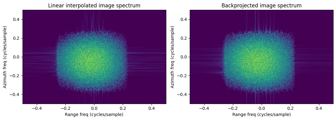
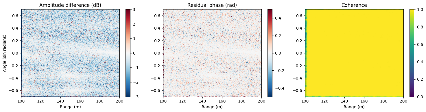
Interpolation kernel

Linear interpolation is much faster, but it also has more interpolation error.

t = time.time()
slave_interp = torchbp.ops.polar_interp(
    slave_own, origin_old=origin_old, origin_new=origin_new,
    grid_polar=grid_polar, fc=fc, rotation=0,
    grid_polar_new=grid_polar, method="linear",
    alias_fmod=alias_fmod)
# polar_interp may return a tuple / extra batch dim; squeeze to 2D
if isinstance(slave_interp, tuple):
    slave_interp = slave_interp[0]
while slave_interp.dim() > 2:
    slave_interp = slave_interp[0]
print(f"polar_interp in {time.time() - t:.3f} s")

polar_interp in 0.004 s

mask = (torch.abs(slave_interp) > 0) & (torch.abs(slave_master) > 0)
b = 20
mask[:b, :] = False; mask[-b:, :] = False
mask[:, :b] = False; mask[:, -b:] = False

phase_res = torch.angle(slave_interp * slave_master.conj())
amp_ratio = torch.abs(slave_interp) / (torch.abs(slave_master) + 1e-10)
coh = torchbp.ops.coherence.coherence_2d(slave_interp, slave_master, (5, 5)).squeeze()

print(f"residual phase : mean {phase_res[mask].mean():+.4f}  std {phase_res[mask].std():.4f} rad")
print(f"amplitude ratio: mean {amp_ratio[mask].mean():.4f}  std {amp_ratio[mask].std():.4f}")
print(f"coherence      : mean {coh[mask].mean():.4f}")

residual phase : mean +0.0000  std 0.1188 rad
amplitude ratio: mean 0.9549  std 0.1484
coherence      : mean 0.9983

fig, axes = plt.subplots(1, 3, figsize=(15, 4))

db_m = 20 * torch.log10(torch.abs(slave_master) + 1e-9)
db_i = 20 * torch.log10(torch.abs(slave_interp) + 1e-9)
im0 = axes[0].imshow((db_i - db_m).cpu().numpy().T, origin="lower", cmap="RdBu_r",
                     vmin=-3, vmax=3, extent=extent, aspect="auto")
axes[0].set_title("Amplitude difference (dB)")
plt.colorbar(im0, ax=axes[0])

im1 = axes[1].imshow(phase_res.cpu().numpy().T, origin="lower", cmap="RdBu_r",
                     vmin=-0.5, vmax=0.5, extent=extent, aspect="auto")
axes[1].set_title("Residual phase (rad)")
plt.colorbar(im1, ax=axes[1])

im2 = axes[2].imshow(coh.cpu().numpy().T, origin="lower", vmin=0, vmax=1,
                     extent=extent, aspect="auto")
axes[2].set_title("Coherence")
plt.colorbar(im2, ax=axes[2])

for ax in axes:
    ax.set_xlabel("Range (m)")
axes[0].set_ylabel("Angle (sin radians)")
plt.tight_layout();

spec_interp_db = 20*np.log10(np.abs(np.fft.fftshift(np.fft.fft2(slave_interp)))).T
m = np.max(spec_interp_db)

fig, axes = plt.subplots(1, 2, figsize=(11, 4))
axes[0].imshow(spec_interp_db, origin="lower", aspect="auto", vmax=m, vmin=m - 40, extent=[-0.5, 0.5, -0.5, 0.5])
axes[0].set_xlabel("Range freq (cycles/sample)")
axes[0].set_ylabel("Azimuth freq (cycles/sample)")
axes[0].set_title("Linear interpolated image spectrum");

axes[1].imshow(spec_master_db, origin="lower", aspect="auto", vmax=m, vmin=m - 40, extent=[-0.5, 0.5, -0.5, 0.5])
axes[1].set_xlabel("Range freq (cycles/sample)")
axes[1].set_ylabel("Azimuth freq (cycles/sample)")
axes[1].set_title("Backprojected image spectrum");
plt.tight_layout();