Cartesian factorized backprojection (CFBP)

Like FFBP (see the ffbp example), CFBP reduces the \(\mathcal{O}(N^2)\) cost of direct backprojection by splitting the aperture into subapertures, imaging each one on a coarse grid, and coherently merging the images in a binary tree. The difference is the grid the factorization runs on:

• FFBP forms each subaperture image on its own local polar grid, centered on the subaperture. Merging requires interpolating between shifted polar frames, a 2D interpolation with a finite kernel (ffbp_merge2).

• CFBP forms every subaperture image on the same global Cartesian grid as the final image, only coarsely sampled in the cross-range direction y. A subaperture image is not bandlimited in y as-is because of the carrier phase \(\exp(j 4\pi f_c d / c)\), but the carrier is a known function of geometry, so it can be removed by multiplying with a reference computed from the subaperture center. The demodulated image is bandlimited, so the coarse y sampling is enough, and since all subimages share the same grid extent, merging only needs interpolation along y-axis plus a phase re-reference.

The library exposes this as a single call, torchbp.ops.cfbp. In this notebook the algorithm is built by hand from backprojection_cart_2d and a few lines of torch to demonstrate how it works.

import math
import torch
import numpy as np
import matplotlib.pyplot as plt
from numpy import hamming

import torchbp
from torchbp.util import center_pos
from torchbp.ops import backprojection_cart_2d

device = "cuda" if torch.cuda.is_available() else "cpu"
print("Device:", device)

Device: cpu

Scene and radar parameters

A single point target imaged on a heavily oversampled Cartesian grid zoomed around the target so the point-spread function (PSF) is smooth and easy to inspect. Same radar parameters as the FFBP example. The platform track is along y (cross-range), boresight along x (range).

fc = 6e9          # RF center frequency (Hz)
bw = 200e6        # RF bandwidth (Hz), positive for rising sweep
tsweep = 100e-6   # Sweep length (s)
fs = 2e6          # Sampling frequency (Hz)
nsweeps = 512     # Number of pulses in the aperture
oversample = 2    # Range FFT oversampling (reduces interpolation error)
nsamples = int(fs * tsweep)

# Heavily oversampled Cartesian grid, zoomed on the target.
nx, ny = 256, 512
grid = {"x": (96.0, 104.0), "y": (-4.0, 4.0), "nx": nx, "ny": ny}

# Single point target at 100 m, broadside.
target_pos = torch.tensor([[100.0, 0.0, 0.0]], dtype=torch.float32, device=device)
target_rcs = torch.ones((1, 1), dtype=torch.float32, device=device)

# Straight platform track along y at 50 m height. Element spacing = lambda/4.
pos = torch.zeros((nsweeps, 3), dtype=torch.float32, device=device)
pos[:, 1] = torch.linspace(-nsweeps / 2, nsweeps / 2, nsweeps, device=device) * 0.25 * 3e8 / fc
pos[:, 2] = 50.0

Simulate and range-compress the data

Identical to the backprojection example. Generate raw data, apply a range window, and FFT to range-compress. data_fmod shifts the data spectrum to DC to reduce the linear interpolation error inside backprojection. Unlike FFBP there is no alias_fmod. The subaperture images are fully demodulated in 2D by the carrier reference, so no separate range-spectrum bookkeeping is needed.

raw = torchbp.util.generate_fmcw_data(target_pos, target_rcs, pos, fc, bw, tsweep, fs)
w = torch.tensor(hamming(raw.shape[-1])[None, :], dtype=torch.float32, device=device)
data = torch.fft.ifft(raw * w, dim=-1, n=nsamples * oversample)

data_fmod = -math.pi * (1 - (oversample - 1) / oversample)
data = data * torch.exp(1j * data_fmod * torch.arange(data.shape[-1], device=device))[None, :]

r_res = 3e8 / (2 * abs(bw) * oversample)  # range bin size in the data
print(f"r_res={r_res:.3f} m, data_fmod={data_fmod:.3f}")

r_res=0.375 m, data_fmod=-1.571

Helpers: display a Cartesian image in dB, and the carrier reference. The image pixel phase is \(\pi k_\text{eff} d\) with \(k_\text{eff} = 4 f_c / c - f_\text{mod} / (\pi \Delta_r)\) (the f_mod term undoes phase of data_fmod term) and \(d\) the distance from the antenna phase center (APC) to the pixel. carrier_ref evaluates \(\exp(\pm j \pi k_\text{eff} d)\) on a grid.

C0 = 299792458.0
keff = 4 * fc / C0 - data_fmod / (math.pi * r_res)

def grid_distance(g, origin, z, dtype=torch.float32):
    x0, x1 = g["x"]; y0, y1 = g["y"]
    dx = (x1 - x0) / g["nx"]; dy = (y1 - y0) / g["ny"]
    # 64-bit precision for more accurate phase computation
    x = x0 - float(origin[0]) + dx * torch.arange(g["nx"], device=device, dtype=torch.float64)
    y = y0 - float(origin[1]) + dy * torch.arange(g["ny"], device=device, dtype=torch.float64)
    d = torch.sqrt(x[:, None] ** 2 + y[None, :] ** 2 + float(z) ** 2)
    return d.to(dtype)

def carrier_ref(g, origin, z, sign):
    d = grid_distance(g, origin, z, dtype=torch.float64)
    ph = torch.remainder(sign * keff * d, 2.0).float() * torch.pi
    return torch.polar(torch.ones_like(ph), ph)

extent = [*grid["y"], *grid["x"]]

def show_cart(img, title, ax=None, dyn=30, ref_max=None):
    img = img.detach().cpu()
    db = 20 * torch.log10(torch.abs(img) + 1e-12)
    m = db.max() if ref_max is None else ref_max
    if ax is None:
        _, ax = plt.subplots()
    im = ax.imshow(db.numpy(), origin="lower", vmin=m - dyn, vmax=m,
                   extent=extent, aspect="auto")
    ax.set_title(title)
    ax.set_xlabel("Cross-range y (m)")
    ax.set_ylabel("Range x (m)")
    return m

def relerr(a, b):
    return (torch.linalg.norm(a - b) / torch.linalg.norm(a)).item()

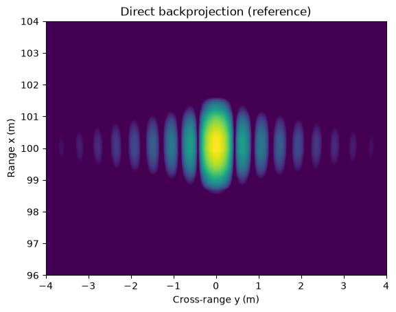
Reference: Direct backprojection

img_bp = backprojection_cart_2d(data, grid, fc, r_res, pos, data_fmod=data_fmod).squeeze(0)

m = show_cart(img_bp, "Direct backprojection (reference)")
plt.show()

Why demodulation is needed

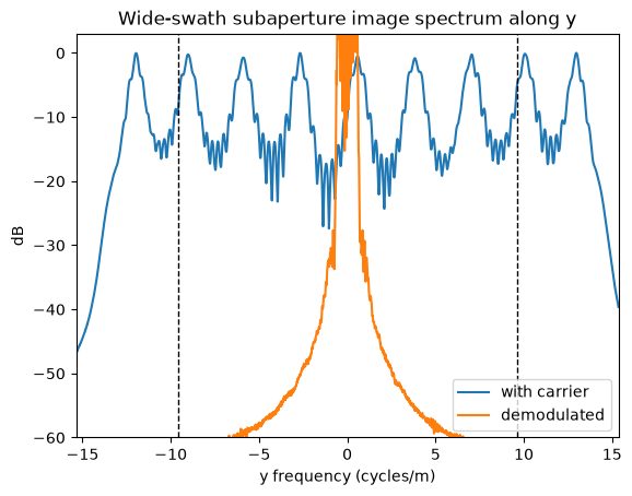
The image carrier has the local y frequency \(k_\text{eff} (y - y_\text{APC}) / (2 d)\) cycles/m at each target, so on a wide swath the carrier spreads the image spectrum far beyond what the coarse subaperture grid can sample. The zoomed single-target grid of this notebook is too small (and too oversampled) to show this, so this cell uses a separate wide demo scene with point targets across the swath. A half-aperture image is formed on a fine grid and its spectrum along y is plotted before and after removing the carrier reference: each target contributes a spectral line at its carrier frequency, and demodulation collapses all of them to baseband, leaving only the subaperture azimuth bandwidth. The dashed lines mark the Nyquist limit of a twice-coarser grid: without demodulation the wide-swath image would alias there, demodulated it fits with a large margin. This is what makes the coarse y sampling of the factorization valid, independent of the scene size.

demo_targets = torch.zeros((9, 3), dtype=torch.float32, device=device)
demo_targets[:, 0] = 100.0
demo_targets[:, 1] = torch.linspace(-36.0, 36.0, 9, device=device)
demo_rcs = torch.ones((9, 1), dtype=torch.float32, device=device)
raw_d = torchbp.util.generate_fmcw_data(demo_targets, demo_rcs, pos, fc, bw, tsweep, fs)
data_d = torch.fft.ifft(raw_d * w, dim=-1, n=nsamples * oversample)
data_d = data_d * torch.exp(1j * data_fmod * torch.arange(data_d.shape[-1], device=device))[None, :]

ny_demo = 3072
grid_demo = {"x": (96.0, 104.0), "y": (-40.0, 40.0), "nx": 128, "ny": ny_demo}

p_half = pos[: nsweeps // 2]
p_local, origin_row = center_pos(p_half)
origin_half = origin_row[0]
z_half = p_half[:, 2].mean()
g_shift = dict(grid_demo,
               x=(grid_demo["x"][0] - float(origin_half[0]), grid_demo["x"][1] - float(origin_half[0])),
               y=(grid_demo["y"][0] - float(origin_half[1]), grid_demo["y"][1] - float(origin_half[1])))
img_half = backprojection_cart_2d(data_d[: nsweeps // 2], g_shift, fc, r_res, p_local,
                                  data_fmod=data_fmod).squeeze(0)
img_half_demod = img_half * carrier_ref(grid_demo, origin_half, z_half, -1.0)

dy_demo = (grid_demo["y"][1] - grid_demo["y"][0]) / ny_demo
fy = np.fft.fftshift(np.fft.fftfreq(ny_demo, d=dy_demo))
spec = lambda im: 20 * np.log10(np.abs(np.fft.fftshift(np.fft.fft(im.cpu().numpy(), axis=-1), axes=-1)).mean(axis=0) + 1e-9)

s0 = spec(img_half); s1 = spec(img_half_demod)
plt.plot(fy, s0 - s0.max(), label="with carrier")
plt.plot(fy, s1 - s0.max(), label="demodulated")
nyq_sub = 1 / (2 * dy_demo * 2)  # Nyquist of a 2x coarser grid
plt.axvline(-nyq_sub, color="k", ls="--", lw=1); plt.axvline(nyq_sub, color="k", ls="--", lw=1)
plt.xlim(-1.6 * nyq_sub, 1.6 * nyq_sub); plt.ylim(-60, 3)
plt.xlabel("y frequency (cycles/m)"); plt.ylabel("dB")
plt.title("Wide-swath subaperture image spectrum along y"); plt.legend(); plt.show()

Step 1: Backproject the subapertures (coarse y)

Split the aperture in two halves. Each half is backprojected with backprojection_cart_2d on the global grid extent with half the y samples, using positions centered on that half’s mean APC (center_pos). The grid is shifted by the same origin, so pixels stay at the same global coordinates. Then the carrier referenced to the subaperture APC is removed. A small internal oversampling factor in y limits the interpolation error in the later merge.

OSR_Y = 1.4  # internal y oversampling of subaperture grids

def backproject_subaperture(sl, ny_sub):
    p = pos[sl]
    p_local, origin_row = center_pos(p)
    origin = origin_row[0]
    z = p[:, 2].mean()
    g = dict(grid, ny=ny_sub)
    g_shift = dict(g,
                   x=(g["x"][0] - float(origin[0]), g["x"][1] - float(origin[0])),
                   y=(g["y"][0] - float(origin[1]), g["y"][1] - float(origin[1])))
    img = backprojection_cart_2d(data[sl], g_shift, fc, r_res, p_local,
                                 data_fmod=data_fmod).squeeze(0)
    img = img * carrier_ref(g, origin, z, -1.0)  # demodulate
    return {"img": img, "grid": g, "origin": origin, "z": z}

half = nsweeps // 2
subA = backproject_subaperture(slice(0, half), int(OSR_Y * ny // 2))
subB = backproject_subaperture(slice(half, nsweeps), int(OSR_Y * ny // 2))

print("subaperture image shape:", tuple(subA["img"].shape), "(full grid is", (nx, ny), ")")
fig, axs = plt.subplots(1, 2, figsize=(11, 4))
show_cart(subA["img"], "Subaperture A (first half)", ax=axs[0])
show_cart(subB["img"], "Subaperture B (second half)", ax=axs[1])
plt.tight_layout(); plt.show()

subaperture image shape: (256, 358) (full grid is (256, 512) )

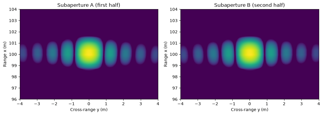
Each subaperture image is focused but the cross-range resolution is half of the reference since only half of the data is used. Unlike FFBP, both images are already in the same global coordinate frame, the target sits at the same (x, y) in both and only the demodulation references differ.

Step 2: Merge

1. Upsample along y to the output grid with FFT zero-padding. Because all grids share the same extent and samples sit at DFT sample positions, this interpolation is exact for the bandlimited demodulated image. torchbp.ops.cfbp also supports faster finite-length interpolation kernel.

2. Re-reference the demodulation carrier from the subaperture APC to the merged APC by multiplying with \(\exp(j \pi k_\text{eff} (d_\text{sub} - d_\text{merged}))\).

3. Sum.

After the final remodulation the result matches direct backprojection up to interpolation error. The upsampler below is the upsampling branch of the library’s torchbp.ops.cfbp._fft_resample_dim.

def fft_upsample_y(img, ny_new):
    ny_old = img.shape[-1]
    if ny_new == ny_old:
        return img
    X = torch.fft.fft(img, dim=-1)
    h = ny_old // 2
    Y = X.new_zeros((*X.shape[:-1], ny_new))
    if ny_old % 2 == 0:
        Y[..., :h] = X[..., :h]
        Y[..., h] = 0.5 * X[..., h]          # split the Nyquist bin
        Y[..., ny_new - h] = 0.5 * X[..., h]
        Y[..., ny_new - h + 1:] = X[..., h + 1:]
    else:
        Y[..., :h + 1] = X[..., :h + 1]
        Y[..., ny_new - h:] = X[..., h + 1:]
    return torch.fft.ifft(Y, dim=-1) * (ny_new / ny_old)

def merge(a, b, ny_new):
    new_origin = 0.5 * (a["origin"] + b["origin"])
    new_z = 0.5 * (a["z"] + b["z"])
    g_new = dict(grid, ny=ny_new)
    d_new = grid_distance(g_new, new_origin, new_z)
    out = 0
    for s in (a, b):
        img = fft_upsample_y(s["img"], ny_new)
        ph = (torch.pi * keff) * (grid_distance(g_new, s["origin"], s["z"]) - d_new)
        out = out + img * torch.polar(torch.ones_like(ph), ph)
    return {"img": out, "grid": g_new, "origin": new_origin, "z": new_z}

merged = merge(subA, subB, ny)
img_cfbp2 = merged["img"] * carrier_ref(grid, merged["origin"], merged["z"], 1.0)  # remodulate

fig, axs = plt.subplots(1, 2, figsize=(11, 4))
show_cart(img_bp, "Direct backprojection", ax=axs[0], ref_max=m)
show_cart(img_cfbp2, "CFBP, 2 subapertures (manual)", ax=axs[1], ref_max=m)
plt.tight_layout(); plt.show()

print(f"relative error vs direct BP: {relerr(img_bp, img_cfbp2):.4f}")

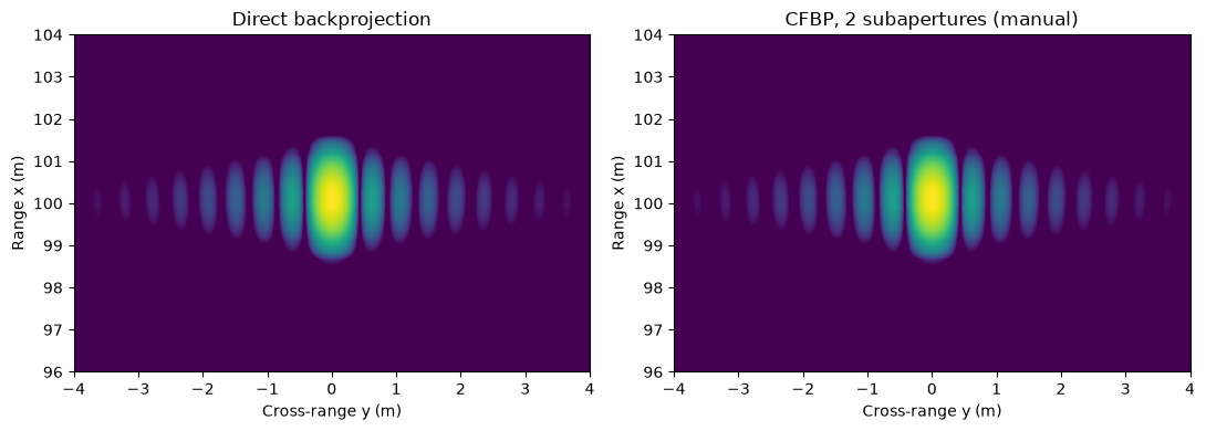
relative error vs direct BP: 0.0009

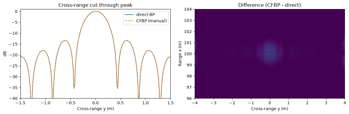
The merged image matches the reference. The cross-range cut through the peak overlays the direct result.

pk = np.unravel_index(torch.abs(img_bp).cpu().argmax(), img_bp.shape)
y_axis = np.linspace(grid["y"][0], grid["y"][1], ny)
cut_bp = 20 * torch.log10(torch.abs(img_bp[pk[0]]).cpu() + 1e-12)
cut_cf = 20 * torch.log10(torch.abs(img_cfbp2[pk[0]]).cpu() + 1e-12)

fig, axs = plt.subplots(1, 2, figsize=(12, 4))
axs[0].plot(y_axis, cut_bp - cut_bp.max(), label="direct BP")
axs[0].plot(y_axis, cut_cf - cut_bp.max(), "--", label="CFBP (manual)")
axs[0].set_xlim(-1.5, 1.5); axs[0].set_ylim(-40, 1)
axs[0].set_xlabel("Cross-range y (m)"); axs[0].set_ylabel("dB")
axs[0].set_title("Cross-range cut through peak"); axs[0].legend()
show_cart(img_bp - img_cfbp2, "Difference (CFBP - direct)", ax=axs[1], ref_max=m, dyn=80)
plt.tight_layout(); plt.show()

/tmp/ipykernel_3613/821849040.py:1: DeprecationWarning: __array__ implementation doesn't accept a copy keyword, so passing copy=False failed. __array__ must implement 'dtype' and 'copy' keyword arguments. To learn more, see the migration guide https://numpy.org/devdocs/numpy_2_0_migration_guide.html#adapting-to-changes-in-the-copy-keyword
  pk = np.unravel_index(torch.abs(img_bp).cpu().argmax(), img_bp.shape)

Recursion

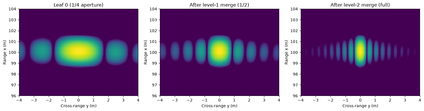
As with FFBP, the real speedup comes from recursing: four subapertures are backprojected on grids with a quarter of the y samples and merged in a two-level binary tree. Each level of the tree doubles the cross-range resolution and the number of y samples.

NSUB = 4
n = nsweeps // NSUB
leaves = [backproject_subaperture(slice(i * n, (i + 1) * n), int(OSR_Y * ny // NSUB))
          for i in range(NSUB)]

# Level 1: merge pairs onto y-oversampled intermediate grids.
mid0 = merge(leaves[0], leaves[1], int(OSR_Y * ny // 2))
mid1 = merge(leaves[2], leaves[3], int(OSR_Y * ny // 2))

# Level 2: merge the intermediates onto the full output grid and remodulate.
merged4 = merge(mid0, mid1, ny)
img_cfbp4 = merged4["img"] * carrier_ref(grid, merged4["origin"], merged4["z"], 1.0)

fig, axs = plt.subplots(1, 3, figsize=(15, 4))
show_cart(leaves[0]["img"], "Leaf 0 (1/4 aperture)", ax=axs[0])
show_cart(mid0["img"], "After level-1 merge (1/2)", ax=axs[1])
show_cart(img_cfbp4, "After level-2 merge (full)", ax=axs[2], ref_max=m)
plt.tight_layout(); plt.show()

print(f"4-subaperture CFBP, relative error vs direct BP: {relerr(img_bp, img_cfbp4):.4f}")

4-subaperture CFBP, relative error vs direct BP: 0.0015

Library op torchbp.ops.cfbp

Everything above is what torchbp.ops.cfbp does internally, plus the y-axis guard band to reduce interpolation error at the edges and support for uneven splits and arbitrary grid sizes. stages is the number of recursion levels.

img_lib1 = torchbp.ops.cfbp(data, grid, fc, r_res, pos, stages=1,
                            data_fmod=data_fmod).squeeze(0)
img_lib2 = torchbp.ops.cfbp(data, grid, fc, r_res, pos, stages=2,
                            data_fmod=data_fmod).squeeze(0)

print(f"stages=1 vs direct BP: {relerr(img_bp, img_lib1):.4f}")
print(f"stages=2 vs direct BP: {relerr(img_bp, img_lib2):.4f}")
print(f"stages=1 vs manual 2-subaperture: {relerr(img_cfbp2, img_lib1):.4f}")
print(f"stages=2 vs manual 4-subaperture: {relerr(img_cfbp4, img_lib2):.4f}")

stages=1 vs direct BP: 0.0016
stages=2 vs direct BP: 0.0029
stages=1 vs manual 2-subaperture: 0.0017
stages=2 vs manual 4-subaperture: 0.0032

Range-adaptive variant torchbp.ops.cfbp_adaptive

A single global stages is wasteful when the scene spans a wide range of ground ranges. The y-bandwidth of a demodulated subaperture grows with the angular extent of the aperture seen from a pixel, which is largest at near range, so the coarsest grid a deep recursion can use is set by the closest range while far ranges could tolerate much deeper factorization. Because the Cartesian scheme never resamples the x (range) axis, the scene can be split into ground-range blocks with no seam error, and each block run at its own y-density and stage count: cfbp_adaptive picks an integer y-oversampling multiplier k(x) and recursion depth s(x) per block, runs the cfbp tree on a grid with k * ny y-samples, and decimates by taking every k-th sample, which lands exactly on the requested output positions. Far ranges keep the full factorization speedup while near ranges automatically fall back to shallower recursion, so the whole image matches direct backprojection to normal CFBP accuracy. stages in this case is the maximum depth.

Benefit and downside

Compared to direct backprojection, CFBP has the same \(\mathcal{O}(N \log N)\) scaling as FFBP. Compared to FFBP it has two attractive properties: the merge interpolation is exact (FFT zero-padding on nested grids) rather than a finite-kernel approximation, and the output is directly on the Cartesian grid with no final polar-to-Cartesian resampling step.

The downside is a geometric one. The demodulated subaperture images contain, in addition to the azimuth bandwidth that shrinks with the subaperture length, the range envelope bandwidth projected onto y, approximately \(\sin(\theta_\text{max}) B\) where \(\theta_\text{max}\) is the largest scene angle from boresight and \(B\) the range bandwidth of the data. This term does not shrink when the aperture is split, so wide angular extents combined with little range oversampling need a larger oversample_y or fewer stages. Polar FFBP does not have this limitation (the envelope varies along its range axis, which is never split), which makes it the better choice for very wide-angle imaging.