Phase gradient autofocus

import torch
import torchbp
import matplotlib.pyplot as plt
from scipy.signal import get_window
import numpy as np

if torch.cuda.is_available():
    device = "cuda"
else:
    device = "cpu"
print("Device:", device)

Device: cpu

Generate synthetic radar data

nr = 100 # Range points
ntheta = 128 # Azimuth points
nsweeps = 128 # Number of measurements
fc = 6e9 # RF center frequency
bw = 100e6 # RF bandwidth
tsweep = 100e-6 # Sweep length
fs = 1e6 # Sampling frequency
nsamples = int(fs * tsweep) # Time domain samples per sweep

# Imaging grid definition. Azimuth angle "theta" is sine of radians. 0.2 = 11.5 degrees.
grid_polar = {"r": (90, 110), "theta": (-0.2, 0.2), "nr": nr, "ntheta": ntheta}

target_pos = torch.tensor([[100, 0, 0], [105, 10, 0], [97, -5, 0], [102, -10, 0], [95, 5, 0]], dtype=torch.float32, device=device)
target_rcs = torch.tensor([1,1,1,1,1], dtype=torch.float32, device=device)

# Slightly non-linear nominal track: non-uniform along-track spacing and
# a known x bow. These are known to the image formation so they don't
# defocus the image.
t = torch.arange(nsweeps, device=device) / nsweeps
pos = torch.zeros([nsweeps, 3], dtype=torch.float32, device=device)
pos[:,1] = torch.linspace(-nsweeps/2, nsweeps/2, nsweeps) * 0.25 * 3e8 / fc * (1 + 0.05 * torch.sin(2 * torch.pi * t))
pos[:,0] = 0.05 * torch.sin(torch.pi * t)

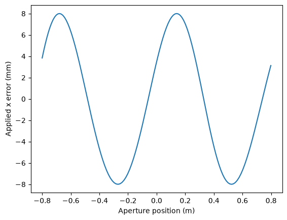
# The true track additionally has an unknown smooth range-direction (x)
# position error, which corrupts the image when the image is formed with
# the nominal track.
dx_true = 8e-3 * torch.sin(2 * torch.pi * 2 * t + 0.5)
pos_true = pos.clone()
pos_true[:,0] += dx_true

plt.figure()
plt.plot(pos[:,1].cpu().numpy(), 1e3 * dx_true.cpu().numpy())
plt.xlabel("Aperture position (m)")
plt.ylabel("Applied x error (mm)");

# Oversampling input data decreases interpolation errors
oversample = 3

# Modulation frequency in range direction to center the spectrum at DC
# for more accurate interpolation.
data_fmod = -torch.pi * (1 - (oversample-1) / oversample)

# Data is simulated at the true track including the position error
data = torchbp.util.generate_fmcw_data(target_pos, target_rcs, pos_true, fc, bw, tsweep, fs)
# Apply windowing function in range direction
wr = torch.tensor(get_window(("taylor", 3, 30), data.shape[-1])[None,:], dtype=torch.float32, device=device)
wa = torch.tensor(get_window(("taylor", 3, 30), data.shape[0])[:,None], dtype=torch.float32, device=device)
data = torch.fft.ifft(data * wa * wr, dim=-1, n=nsamples * oversample)

data_fmod_f = torch.exp(1j*data_fmod*torch.arange(data.shape[-1], device=device))[None,:]
data = data * data_fmod_f

data_db = 20*torch.log10(torch.abs(data)).detach()
m = torch.max(data_db)

plt.figure()
plt.imshow(data_db.cpu().numpy(), origin="lower", vmin=m-30, vmax=m, aspect="auto")
plt.xlabel("Range samples")
plt.ylabel("Azimuth samples");

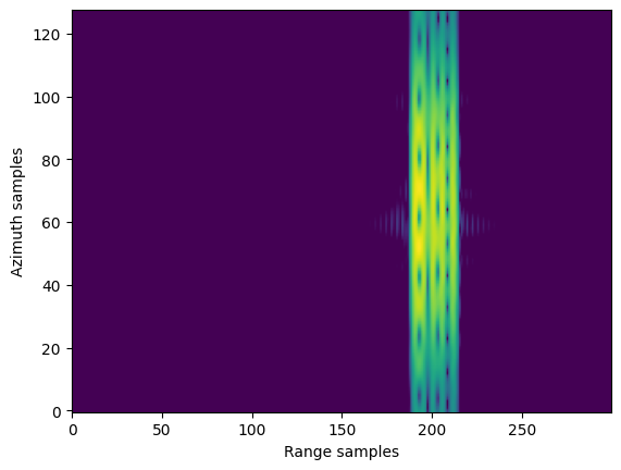
Reference image formed with the true track. The position error is included in the imaging, so nothing defocuses.

r_res = 3e8 / (2 * bw * oversample) # Range bin size in input data

# dealias=True removes range spectrum aliasing
img = torchbp.ops.backprojection_polar_2d(data, grid_polar, fc, r_res, pos_true, dealias=True, data_fmod=data_fmod)
img = img.squeeze(0) # Removes singular batch dimension
# Backprojection image has spectrum with DC at zero index.
# Shifting the spectrum shifts the DC to center bin.
# This makes the solved phase to have same order as the position vector
# Without shifting of the image, fftshift needs to be applied to
# the solved phase for it to be in the same order as the position vector.
# This doesn't affect the absolute value of the image.
img = torchbp.util.shift_spectrum(img)

img_db = 20*torch.log10(torch.abs(img)).detach()

m = torch.max(img_db)

extent = [*grid_polar["r"], *grid_polar["theta"]]

plt.figure()
plt.imshow(img_db.cpu().numpy().T, origin="lower", vmin=m-40, vmax=m, extent=extent, aspect="auto")
plt.xlabel("Range (m)")
plt.ylabel("Angle (sin radians)");

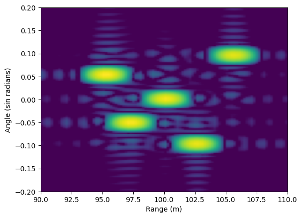
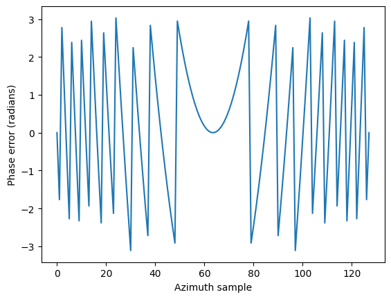
Corrupted image formed with the nominal track. The unaccounted x position error creates a smooth per-sweep phase error that defocuses the image in the azimuth direction. On this narrow scene the phase error is 4*pi/wl * dx since the elevation angle is zero and the scene is centered at broadside.

img_corrupted = torchbp.ops.backprojection_polar_2d(data, grid_polar, fc, r_res, pos, dealias=True, data_fmod=data_fmod)
img_corrupted = img_corrupted.squeeze(0)
img_corrupted = torchbp.util.shift_spectrum(img_corrupted)

# Equivalent per-sweep phase error caused by the x position error
wl = 3e8 / fc
phase_error_true = 4 * torch.pi / wl * dx_true

plt.figure()
plt.plot(pos[:,1].cpu().numpy(), phase_error_true.cpu().numpy())
plt.xlabel("Aperture position (m)")
plt.ylabel("Phase error (radians)")

plt.figure()
plt.imshow(20*torch.log10(torch.abs(img_corrupted)).cpu().numpy().T, origin="lower", vmin=m-40, vmax=m, extent=extent, aspect="auto")
plt.xlabel("Range (m)")
plt.ylabel("Angle (sin radians)");

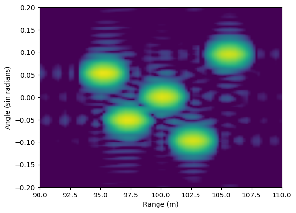
Phase gradient autofocus with phase difference estimator

img_pga, phi = torchbp.autofocus.pga(img_corrupted, estimator="pd")

plt.figure()
plt.imshow(20*torch.log10(torch.abs(img_pga)).cpu().numpy().T, origin="lower", vmin=m-40, vmax=m, extent=extent, aspect="auto")
plt.xlabel("Range (m)")
plt.ylabel("Angle (sin radians)");

plt.figure()
plt.plot(torch.angle(torch.exp(1j*phi)).cpu().numpy())
plt.xlabel("Azimuth samples")
plt.ylabel("Phase error (radians)");

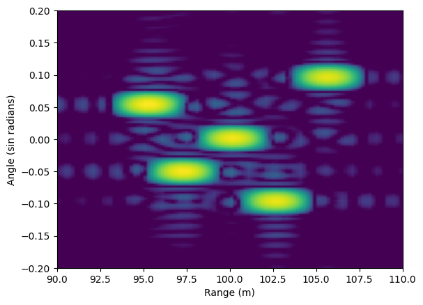
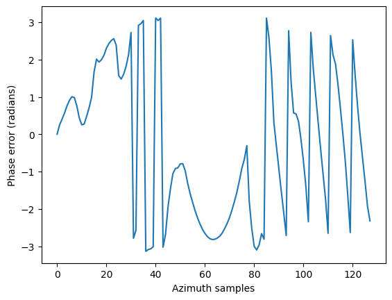
Apply maximum likelihood phase gradient autofocus

img_pga, phi = torchbp.autofocus.pga(img_corrupted, estimator="ml")

plt.figure()
plt.imshow(20*torch.log10(torch.abs(img_pga)).cpu().numpy().T, origin="lower", vmin=m-40, vmax=m, extent=extent, aspect="auto")
plt.xlabel("Range (m)")
plt.ylabel("Angle (sin radians)");

plt.figure()
plt.plot(torch.angle(torch.exp(1j*phi)).cpu().numpy())
plt.xlabel("Azimuth samples")
plt.ylabel("Phase error (radians)");

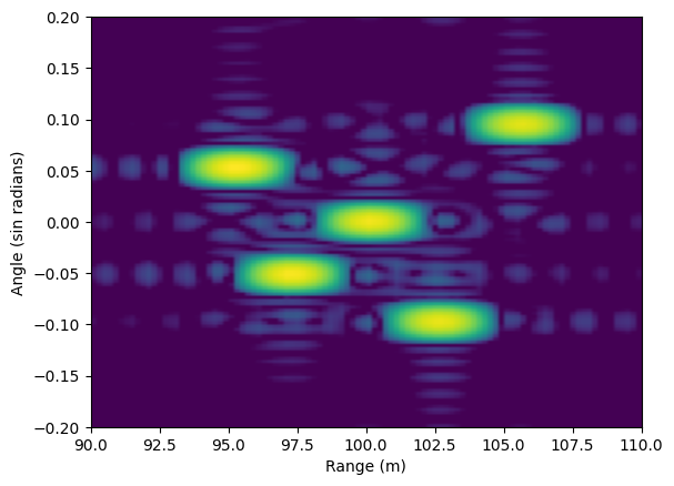
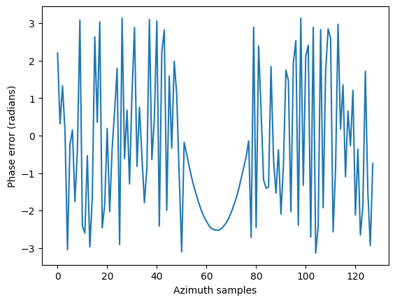
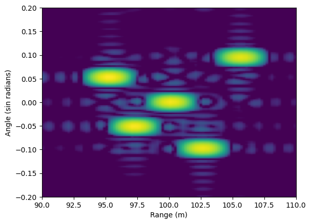
Weighted least squares estimator. This is the default estimator. It weights each range bin by its estimated signal-to-clutter ratio, which usually gives the most accurate estimate when the image has both strong point-like targets and clutter. Not much difference in this case because it’s clutter and noise free.

img_pga, phi = torchbp.autofocus.pga(img_corrupted, estimator="wls")

plt.figure()
plt.imshow(20*torch.log10(torch.abs(img_pga)).cpu().numpy().T, origin="lower", vmin=m-40, vmax=m, extent=extent, aspect="auto")
plt.xlabel("Range (m)")
plt.ylabel("Angle (sin radians)");

plt.figure()
plt.plot(torch.angle(torch.exp(1j*phi)).cpu().numpy())
plt.xlabel("Azimuth samples")
plt.ylabel("Phase error (radians)");

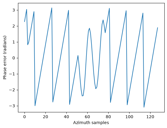
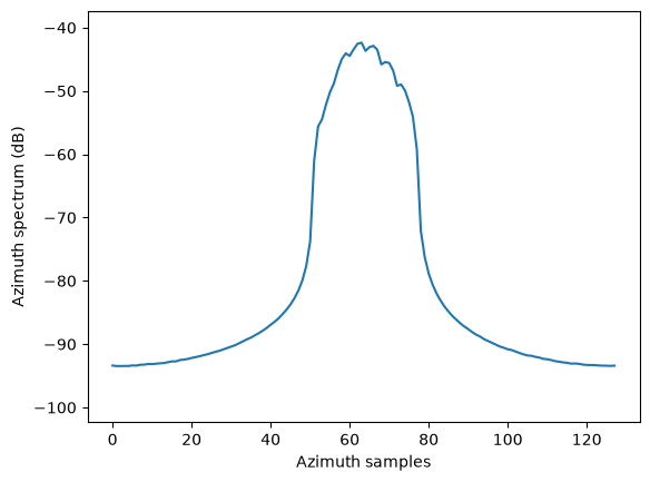
The solved phase is only meaningful over the occupied part of the azimuth spectrum. The width of the spectrum is set by the aperture length and since the theta axis is oversampled, the spectrum only fills a part of the full azimuth extent (it is centered because of the shift_spectrum call above). The phase error and the PGA correction multiply this spectrum, so only the phase over the occupied center bins has any effect on the image. Away from the spectrum there is no signal constraining the estimate. By default pga measures the spectrum support (spectrum_support argument) and restricts the estimators and the linear trend removal to the occupied bins. Without the gating the noise-only bins would corrupt the estimator statistics and bias the trend removal, which would shift the image.

spectrum = torch.fft.fft(img_corrupted, dim=-1)
spectrum_db = 20*torch.log10(torch.mean(torch.abs(spectrum), dim=0))
m_s = torch.max(spectrum_db).item()

plt.figure()
plt.plot(spectrum_db.cpu().numpy())
plt.ylim(m_s - 60, m_s + 5)
plt.xlabel("Azimuth samples")
plt.ylabel("Azimuth spectrum (dB)");

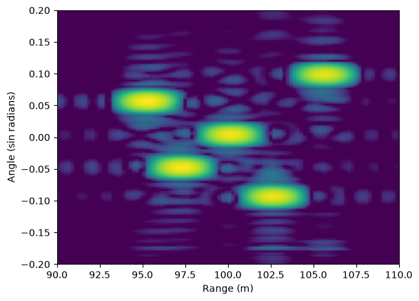
Multiplying the FFT of the corrupted image with the solved phase and taking inverse FFT gives the focused image. This should be identical to the image returned by pga.

img_focused = torch.fft.ifft(torch.fft.fft(img_corrupted, dim=-1) * torch.exp(-1j*phi), dim=-1)

plt.figure()
plt.imshow(20*torch.log10(torch.abs(img_focused)).cpu().numpy().T, origin="lower", vmin=m-40, vmax=m, extent=extent, aspect="auto")
plt.xlabel("Range (m)")
plt.ylabel("Angle (sin radians)");

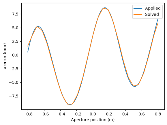
The solved phase can be converted back to a range-direction (x) position error with phase_to_pos. Linear error which can’t be solved by pga is removed both from true and solved position.

dx_solved = torchbp.autofocus.phase_to_pos(phi, grid_polar, fc, pos)

u = pos[:,1].cpu().numpy()

def detrend_on_track(x, u):
    return x - np.polyval(np.polyfit(u, x, 1), u)

plt.figure()
plt.plot(u, 1e3 * detrend_on_track(dx_true.cpu().numpy(), u), label="Applied")
plt.plot(u, 1e3 * detrend_on_track(dx_solved.cpu().numpy(), u), label="Solved")
plt.legend()
plt.xlabel("Aperture position (m)")
plt.ylabel("x error (mm)");

CFBP + PGA

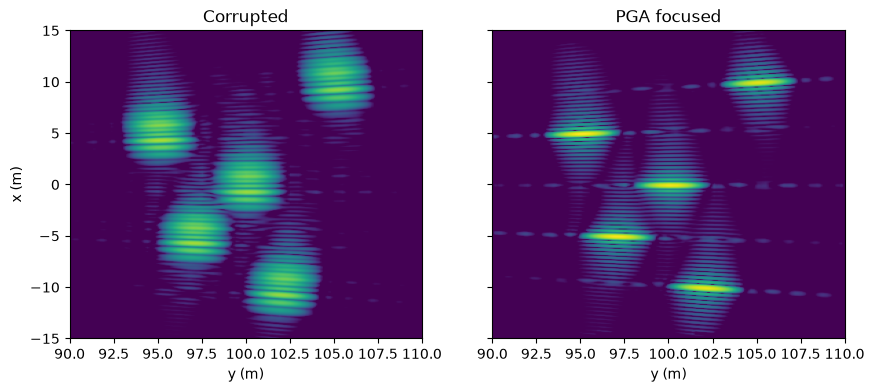
PGA assumes an image in polar geometry where the azimuth phase error is a multiplicative function of the azimuth spectrum. A Cartesian image, for example from cfbp (Cartesian factored backprojection), does not satisfy this assumption, but it can be resampled to a polar grid with cart_to_polar, focused with PGA, and resampled back with polar_to_cart.

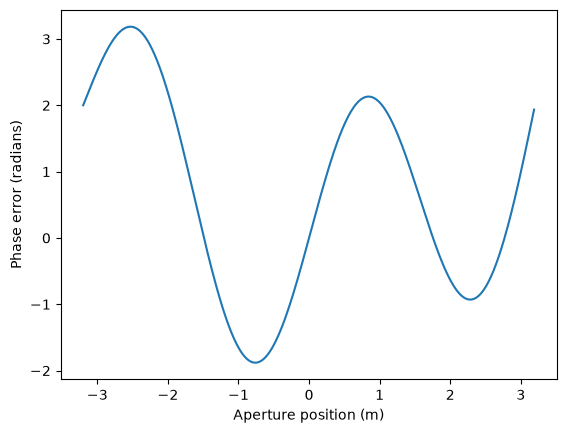
This time the phase error is applied to the raw data with one phase value per sweep, which is how an error from motion measurement inaccuracy would appear.

nsweeps_cfbp = 512
pos_cfbp = torch.zeros([nsweeps_cfbp, 3], dtype=torch.float32, device=device)
pos_cfbp[:,1] = 0.25 * 3e8 / fc * (torch.arange(nsweeps_cfbp, device=device) - nsweeps_cfbp / 2)

data_cfbp = torchbp.util.generate_fmcw_data(target_pos, target_rcs, pos_cfbp, fc, bw, tsweep, fs)
data_cfbp = torch.fft.ifft(data_cfbp * wr, dim=-1, n=nsamples * oversample)
data_cfbp = data_cfbp * data_fmod_f

# Smooth per-sweep phase error
t = torch.arange(nsweeps_cfbp, device=device) / nsweeps_cfbp
phase_error_sweep = 2 * torch.sin(2 * torch.pi * 2 * t) + 8 * (t - 0.5)**2
data_corrupted = data_cfbp * torch.exp(1j * phase_error_sweep)[:, None]

plt.figure()
plt.plot(pos_cfbp[:,1].cpu().numpy(), phase_error_sweep.cpu().numpy())
plt.xlabel("Aperture position (m)")
plt.ylabel("Phase error (radians)");

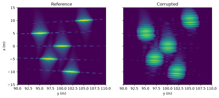
Reference and corrupted Cartesian images with CFBP.

grid_cart = {"x": (90, 110), "y": (-15, 15), "nx": 256, "ny": 384}

img_cart_ref = torchbp.ops.cfbp(data_cfbp, grid_cart, fc, r_res, pos_cfbp, stages=3, data_fmod=data_fmod)[0]
img_cart_corrupted = torchbp.ops.cfbp(data_corrupted, grid_cart, fc, r_res, pos_cfbp, stages=3, data_fmod=data_fmod)[0]

extent_cart = [*grid_cart["x"], *grid_cart["y"]]
m_cart = 20*torch.log10(torch.max(torch.abs(img_cart_ref))).item()

fig, axes = plt.subplots(1, 2, figsize=(10, 4), sharey=True)
for ax, img_i, title in zip(axes, (img_cart_ref, img_cart_corrupted), ("Reference", "Corrupted")):
    img_db_i = 20*torch.log10(torch.abs(img_i))
    ax.imshow(img_db_i.cpu().numpy().T, origin="lower", vmin=m_cart-40, vmax=m_cart, extent=extent_cart, aspect="auto")
    ax.set_title(title)
    ax.set_xlabel("y (m)")
axes[0].set_ylabel("x (m)");

Resample the corrupted image to a polar grid centered on the aperture center. cart_to_polar removes the range carrier during the interpolation, so the output is equivalent to a dealiased polar image from backprojection. The polar grid needs to cover the Cartesian grid as seen from the origin, theta needs to sample the azimuth bandwidth of the full aperture and r the range envelope bandwidth of the data. shift_spectrum centers the azimuth spectrum like before.

origin_cfbp = torch.mean(pos_cfbp, axis=0)
grid_polar_cfbp = {"r": (89, 112), "theta": (-0.18, 0.18), "nr": 192, "ntheta": 256}

img_polar = torchbp.ops.cart_to_polar(img_cart_corrupted, origin_cfbp, grid_cart, grid_polar_cfbp, fc, method=("lanczos", 8))[0]
img_polar = torchbp.util.shift_spectrum(img_polar)

extent_polar = [*grid_polar_cfbp["r"], *grid_polar_cfbp["theta"]]
img_polar_db = 20*torch.log10(torch.abs(img_polar))

plt.figure()
plt.imshow(img_polar_db.cpu().numpy().T, origin="lower", vmin=m_cart-40, vmax=m_cart, extent=extent_polar, aspect="auto")
plt.xlabel("Range (m)")
plt.ylabel("Angle (sin radians)");

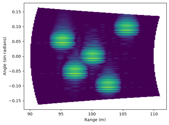
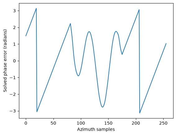
Apply PGA on the polar image with the default settings (weighted least squares estimator with trend removal). The solved phase over the occupied center bins resembles the applied phase error with its linear trend removed. The trend is unobservable to PGA and removing it keeps the image from shifting.

img_polar_pga, phi = torchbp.autofocus.pga(img_polar)

plt.figure()
plt.plot(torch.angle(torch.exp(1j*phi)).cpu().numpy())
plt.xlabel("Azimuth samples")
plt.ylabel("Solved phase error (radians)");

Undo the spectrum shift and resample the focused polar image back to the Cartesian grid. The shift needs to be undone because polar_to_cart interpolates the image and the shift modulates the image at the azimuth Nyquist frequency, which would make it too high frequency to interpolate.

img_polar_pga = torchbp.util.shift_spectrum(img_polar_pga)
img_cart_pga = torchbp.ops.polar_to_cart(img_polar_pga, origin_cfbp, grid_polar_cfbp, grid_cart, fc, method=("lanczos", 8))[0]

fig, axes = plt.subplots(1, 2, figsize=(10, 4), sharey=True)
for ax, img_i, title in zip(axes, (img_cart_corrupted, img_cart_pga), ("Corrupted", "PGA focused")):
    img_db_i = 20*torch.log10(torch.abs(img_i))
    ax.imshow(img_db_i.cpu().numpy().T, origin="lower", vmin=m_cart-40, vmax=m_cart, extent=extent_cart, aspect="auto")
    ax.set_title(title)
    ax.set_xlabel("y (m)")
axes[0].set_ylabel("x (m)");

Range and elevation dependent autofocus

pga solves a single phase error profile that is applied uniformly to every range bin. A platform position error, however, creates a phase error that depends on the look direction to each pixel: a vertical (z) position error contributes proportionally to the sine of the elevation angle and a range direction (x) error proportionally to its cosine. When the platform altitude is comparable to the range extent, the elevation angle changes over the range swath and no single phase profile can focus the whole image.

pga_xz estimates the range-direction (x) and vertical (z) platform position error profiles by running the PGA estimator on blocks of range rows and solving the two components for each azimuth spectrum bin from the block phases. The correction is applied with per-row multiplies in the azimuth spectrum domain, so like pga it runs entirely on the image with FFTs and needs no raw data. See gpga_tde for the data domain equivalent that also estimates the along-track error component and re-forms the image with the corrected trajectory.

The scene: platform at 50 m altitude imaging a 50-120 m ground range swath, so the elevation angle varies from 45 to 23 degrees over the image. A longer aperture than before is used to get a wider azimuth spectrum. The platform track has smooth x and z position errors.

h = 50.0 # Platform altitude
nsweeps_xz = 512
grid_xz = {"r": (50, 120), "theta": (-0.2, 0.2), "nr": 128, "ntheta": 256}

torch.manual_seed(123)
ntargets = 20
tr = 55.0 + 60.0 * torch.rand(ntargets, device=device)
tt = -0.15 + 0.3 * torch.rand(ntargets, device=device)
targets_xz = torch.stack([tr * torch.sqrt(1 - tt**2), tr * tt, torch.zeros_like(tr)], dim=1)
rcs_xz = torch.ones(ntargets, dtype=torch.complex64, device=device)

pos_xz = torch.zeros([nsweeps_xz, 3], dtype=torch.float32, device=device)
pos_xz[:,1] = 0.25 * 3e8 / fc * (torch.arange(nsweeps_xz, device=device) - nsweeps_xz / 2)
pos_xz[:,2] = h

# True track has smooth x and z position errors
t_xz = torch.arange(nsweeps_xz, device=device) / nsweeps_xz
dx_true = 5e-3 * torch.sin(2 * torch.pi * 2 * t_xz + 0.5)
dz_true = 20e-3 * torch.sin(2 * torch.pi * 3 * t_xz + 1.0)
pos_true = pos_xz.clone()
pos_true[:,0] += dx_true
pos_true[:,2] += dz_true

plt.figure()
plt.plot(pos_xz[:,1].cpu().numpy(), 1e3 * dx_true.cpu().numpy(), label="x error")
plt.plot(pos_xz[:,1].cpu().numpy(), 1e3 * dz_true.cpu().numpy(), label="z error")
plt.legend()
plt.xlabel("Aperture position (m)")
plt.ylabel("Position error (mm)");

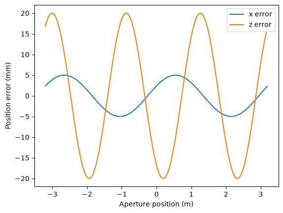
The data is simulated at the true positions and the image is formed at the nominal straight track, which defocuses the image. Note that shift_spectrum is not applied this time: pga_xz centers the azimuth spectrum internally and expects the image straight from backprojection (spectrum DC at zero index), because its per-row spectral scaling is anchored at zero azimuth frequency. pga is indifferent to the spectrum position: its spectrum support gating finds the occupied band wherever it is, so it works identically on the shifted and non-shifted image. Shifting only changes the bin ordering of its returned phase, which is not used here.

data_xz = torchbp.util.generate_fmcw_data(targets_xz, rcs_xz, pos_true, fc, bw, tsweep, fs)
wa_xz = torch.tensor(get_window(("taylor", 3, 30), nsweeps_xz)[:,None], dtype=torch.float32, device=device)
data_xz = torch.fft.ifft(data_xz * wa_xz * wr, dim=-1, n=nsamples * oversample)
data_xz = data_xz * data_fmod_f

img_ref_xz = torchbp.ops.backprojection_polar_2d(data_xz, grid_xz, fc, r_res, pos_true, dealias=True, data_fmod=data_fmod)[0]
img_corrupted_xz = torchbp.ops.backprojection_polar_2d(data_xz, grid_xz, fc, r_res, pos_xz, dealias=True, data_fmod=data_fmod)[0]

extent_xz = [*grid_xz["r"], *grid_xz["theta"]]
m_xz = 20*torch.log10(torch.max(torch.abs(img_ref_xz))).item()

fig, axes = plt.subplots(1, 2, figsize=(10, 4), sharey=True)
for ax, img_i, title in zip(axes, (img_ref_xz, img_corrupted_xz), ("Ideal image", "Corrupted image")):
    img_db_i = 20*torch.log10(torch.abs(img_i))
    ax.imshow(img_db_i.cpu().numpy().T, origin="lower", vmin=m_xz-40, vmax=m_xz, extent=extent_xz, aspect="auto")
    ax.set_title(title)
    ax.set_xlabel("Range (m)")
axes[0].set_ylabel("Angle (sin radians)");

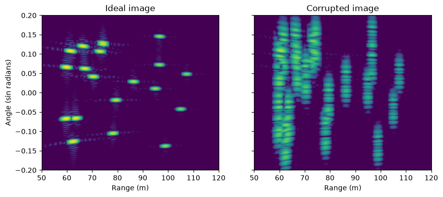
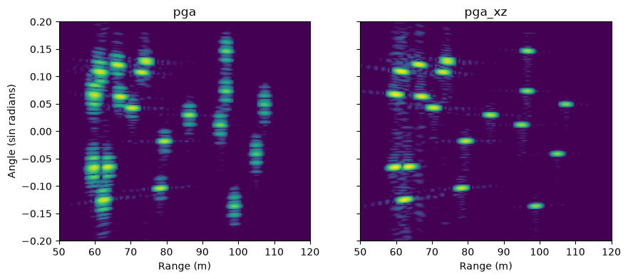
Plain pga solves the best single phase profile. It focuses the image where the elevation angle matches the average, but the z error contribution scales with the sine of the elevation angle, so single phase correction over the whole image can’t focus all targets at the same time.

img_pga_1d, phi_1d = torchbp.autofocus.pga(img_corrupted_xz)

plt.figure()
plt.imshow(20*torch.log10(torch.abs(img_pga_1d)).cpu().numpy().T, origin="lower", vmin=m_xz-40, vmax=m_xz, extent=extent_xz, aspect="auto")
plt.xlabel("Range (m)")
plt.ylabel("Angle (sin radians)");

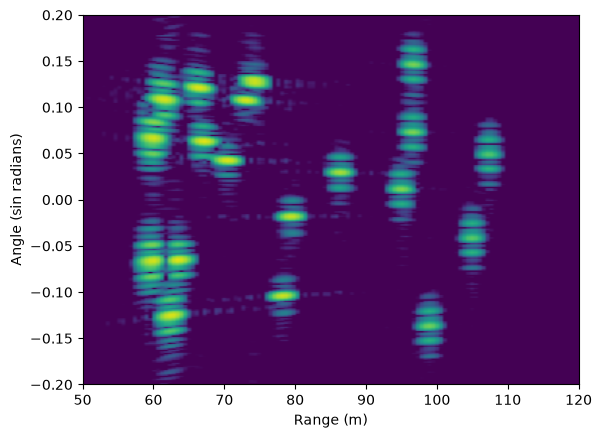
pga_xz needs the grid and the platform altitude for the per-row elevation angle and the number of range blocks to estimate from.

img_pga_xz, d_xz = torchbp.autofocus.pga_xz(img_corrupted_xz, grid_xz, fc, h, range_divisions=4)

fig, axes = plt.subplots(1, 2, figsize=(10, 4), sharey=True)
for ax, img_i, title in zip(axes, (img_pga_1d, img_pga_xz), ("pga", "pga_xz")):
    img_db_i = 20*torch.log10(torch.abs(img_i))
    ax.imshow(img_db_i.cpu().numpy().T, origin="lower", vmin=m_xz-40, vmax=m_xz, extent=extent_xz, aspect="auto")
    ax.set_title(title)
    ax.set_xlabel("Range (m)")
axes[0].set_ylabel("Angle (sin radians)");

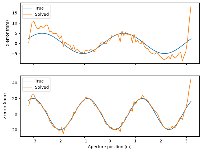
pga_xz returns the solved x and z position error profiles in meters as a function of the fftshifted azimuth spectrum bin. For comparison against the original error the mapping from spectrum to along-track position needs to be applied. This mapping is not needed by the correction itself, only to compare against the true error. The profiles are only meaningful over the occupied part of the spectrum, i.e. aperture positions inside the actual track, and the mean and linear trend are unobservable to PGA and removed.

ntheta_xz = grid_xz["ntheta"]
dtheta_xz = (grid_xz["theta"][1] - grid_xz["theta"][0]) / ntheta_xz
wl = 3e8 / fc
cos_el_ref = grid_xz["r"][1] / np.hypot(grid_xz["r"][1], h)
bins_xz = torch.arange(ntheta_xz, device=device) - ntheta_xz // 2
u_xz = -bins_xz * wl / (2 * cos_el_ref * dtheta_xz * ntheta_xz)

# Keep only the bins that map to positions inside the actual aperture,
# the profile outside the occupied spectrum is not meaningful.
in_aperture = torch.abs(u_xz) <= torch.max(torch.abs(pos_xz[:,1]))

fig, axes = plt.subplots(2, 1, figsize=(8, 6), sharex=True)
for ax, d_i, true_i, name in zip(axes, d_xz, (dx_true, dz_true), ("x", "z")):
    ax.plot(pos_xz[:,1].cpu().numpy(), 1e3 * true_i.cpu().numpy(), label="True")
    ax.plot(u_xz[in_aperture].cpu().numpy(), 1e3 * d_i[in_aperture].cpu().numpy(), label="Solved")
    ax.set_ylabel(f"{name} error (mm)")
    ax.legend()
axes[-1].set_xlabel("Aperture position (m)");

Antenna-weighted PGA (stripmap)

Everything above assumed a spotlight-like collection: every target is visible over the whole aperture, so every azimuth spectrum bin of every target carries signal. In a stripmap collection a narrow azimuth beam sweeps over the scene and each target is illuminated for only part of the aperture. Each target then occupies only its own sub-band of the azimuth spectrum, and for every target the bins outside its sub-band hold unrelated clutter from the same range, which corrupts the estimate.

pga fixes this when given the same antenna model the imaging operators use (the grid, fc, pos, att, g and g_extent arguments). It then computes for every selected target the two-way antenna amplitude at the pulse that illuminated each spectrum bin and weights the estimator with it.

The scene setup follows the antenna_normalization example: a straight track along \(y\) at 30 m altitude with a narrow 4 degree azimuth beam. The beam footprint at mid swath is about 13 m while the track is 25.6 m, so targets continuously enter and leave the beam. A smooth range-direction position error is injected like before.

torch.manual_seed(0)

fc_sm = 6e9
bw_sm = 200e6
tsweep_sm = 100e-6
fs_sm = 5e6
nsamples_sm = int(fs_sm * tsweep_sm)
nsweeps_sm = 1024
wl = 3e8 / fc_sm
altitude_sm = 30.0

pos_sm = torch.zeros([nsweeps_sm, 3], dtype=torch.float32, device=device)
pos_sm[:,1] = 0.5 * wl * (torch.arange(nsweeps_sm, device=device) - nsweeps_sm / 2)
pos_sm[:,2] = altitude_sm
track_sm = nsweeps_sm * 0.5 * wl

# Narrow azimuth beam, wide elevation beam rolled down to mid swath.
az_sm = np.linspace(-np.pi/6, np.pi/6, 128)
el_sm = np.linspace(-np.pi/3, np.pi/3, 64)
gain_sm = np.exp(-(el_sm[:,None] / np.deg2rad(25.0))**2) \
    * np.exp(-(az_sm[None,:] / np.deg2rad(4.0))**2)
g_sm = torch.tensor(gain_sm, dtype=torch.float32, device=device)
g_extent_sm = [el_sm[0], az_sm[0], el_sm[-1], az_sm[-1]]

r_mid_sm = 75.0
att_sm = torch.zeros_like(pos_sm)
att_sm[:,0] = -np.arctan2(altitude_sm, r_mid_sm)

# Smooth range (x) position error, rms about half a wavelength.
t_sm = torch.arange(nsweeps_sm, dtype=torch.float32, device=device) / nsweeps_sm
dx_sm = 0.03 * torch.sin(2*torch.pi*2.5*t_sm) \
    + 0.015 * torch.sin(2*torch.pi*5.5*t_sm + 1.0)
pos_true_sm = pos_sm.clone()
pos_true_sm[:,0] += dx_sm

print(f"Track {track_sm:.1f} m, injected x error rms "
      f"{1e3 * dx_sm.pow(2).mean().sqrt():.1f} mm")

Track 25.6 m, injected x error rms 23.7 mm

The scene is a row of unit point targets spaced 5 m along the track, less than the beam footprint, so at least one target is in the beam at every sweep. The raw data is simulated along the true trajectory with projection_cart_2d_nufft, weighting every scatterer with the antenna pattern, and range-compressed with a Hamming window as in the antenna_normalization example.

grid_proj_sm = {"x": (45.0, 105.0), "y": (-25.0, 25.0), "nx": 512, "ny": 512}
dxp = (grid_proj_sm["x"][1] - grid_proj_sm["x"][0]) / grid_proj_sm["nx"]
dyp = (grid_proj_sm["y"][1] - grid_proj_sm["y"][0]) / grid_proj_sm["ny"]
scene_sm = 0.004 * torch.randn([grid_proj_sm["nx"], grid_proj_sm["ny"]],
                               dtype=torch.complex64, device=device)

ty_sm = np.arange(-17.5, 18.0, 5.0)
tx_sm = np.array([62.0, 80.0, 70.0, 88.0, 65.0, 84.0, 74.0, 91.0])
targets_sm = []
for k in range(len(tx_sm)):
    i = int(round((tx_sm[k] - grid_proj_sm["x"][0]) / dxp))
    j = int(round((ty_sm[k] - grid_proj_sm["y"][0]) / dyp))
    scene_sm[i, j] = 1.0
    # Remember the pixel-center position actually simulated.
    targets_sm.append([grid_proj_sm["x"][0] + dxp * i,
                       grid_proj_sm["y"][0] + dyp * j])
targets_sm = np.array(targets_sm)

oversample_sm = 2
data_fmod_sm = -torch.pi * (1 - (oversample_sm - 1) / oversample_sm)
r_res_sm = 3e8 / (2 * bw_sm * oversample_sm)

data_sm = torchbp.ops.projection_cart_2d_nufft(
    scene_sm, pos_true_sm, grid_proj_sm, fc_sm, fs_sm, bw_sm / tsweep_sm,
    nsamples_sm, att=att_sm, g=g_sm, g_extent=g_extent_sm, use_rvp=False,
    normalization="sigma")[0]
wr_sm = torch.tensor(get_window("hamming", data_sm.shape[-1])[None,:],
                     dtype=torch.float32, device=device)
data_sm = torch.fft.ifft(data_sm * wr_sm, dim=-1, n=nsamples_sm * oversample_sm)
data_sm = data_sm * torch.exp(
    1j * data_fmod_sm * torch.arange(data_sm.shape[-1], device=device))[None,:]

One grid detail matters here. The azimuth spectrum bins of a polar image map to along-track platform positions, and the whole spectrum spans an aperture of

\[L_\mathrm{spec} = \frac{\lambda}{2 \cos(\mathrm{el}) \, d\theta}\]

meters. If this is shorter than the flown track the aperture aliases in the spectrum, every target smears over all bins and image-domain PGA cannot work at all. ntheta has to be chosen large enough (azimuth oversampled) that the spectrum holds the track.

theta_limit_sm = 0.42
ntheta_sm = 1024
dtheta_sm = 2 * theta_limit_sm / ntheta_sm
grid_sm = {"r": (50.0, 100.0), "theta": (-theta_limit_sm, theta_limit_sm),
           "nr": 96, "ntheta": ntheta_sm}

cos_el_sm = r_mid_sm / np.hypot(r_mid_sm, altitude_sm)
print(f"Spectrum span: {wl / (2 * cos_el_sm * dtheta_sm):.1f} m, "
      f"track: {track_sm:.1f} m")

Spectrum span: 32.8 m, track: 25.6 m

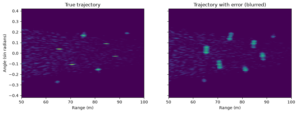
Backprojecting with the nominal trajectory defocuses the targets, the reference formed with the true trajectory shows what autofocus should recover. Both are formed with the antenna pattern, the same way the autofocus later models the illumination.

def form_image_sm(p):
    return torchbp.ops.backprojection_polar_2d(
        data_sm, grid_sm, fc_sm, r_res_sm, p, data_fmod=data_fmod_sm,
        att=att_sm, g=g_sm, g_extent=g_extent_sm)[0]

img_blur_sm = form_image_sm(pos_sm)
img_true_sm = form_image_sm(pos_true_sm)

extent_sm = [*grid_sm["r"], *grid_sm["theta"]]
m_sm = 20 * torch.log10(torch.abs(img_true_sm)).max().item()

def show_sm(ax, img_i, title):
    db_i = 20 * torch.log10(torch.abs(img_i) + 1e-12)
    ax.imshow(db_i.cpu().numpy().T, origin="lower", vmin=m_sm-35, vmax=m_sm,
              extent=extent_sm, aspect="auto")
    ax.set_title(title)
    ax.set_xlabel("Range (m)")

fig, axes = plt.subplots(1, 2, figsize=(12, 4), sharey=True)
show_sm(axes[0], img_true_sm, "True trajectory")
show_sm(axes[1], img_blur_sm, "Trajectory with error (blurred)")
axes[0].set_ylabel("Angle (sin radians)");

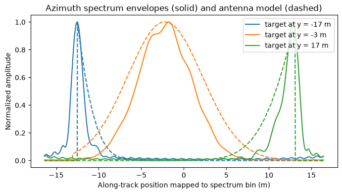
To see why plain pga struggles here, window a few targets out of the focused image and look at their azimuth spectra. Each target’s spectrum is occupied only where the beam illuminated it, and since the targets sit at different along-track positions the occupied sub-bands are different. The dashed lines show the illumination predicted by the antenna model, the weights the antenna-weighted pga uses internally (computed by its _antenna_spectrum_weights helper). Plain pga weights all bins of a target equally, so for every target most of the spectrum contributes only clutter.

The model and the measurement differ in two visible ways, neither of which affects the autofocus. At the track ends the dashed model drops to zero abruptly, because bins mapping to along-track positions beyond the flown track get exactly zero weight, since no pulses exist there. The data support ends just as abruptly, but the measured envelope cannot show it and the image domain has smoother roll-off. At the center, the measurement falls below the model. The image was formed with the antenna pattern, and antenna-weighted backprojection is a matched filter that weights each pulse by g again on data that is already proportional to g, so the image spectrum rolls off as g^2 while the dashed model is g. Weighting the estimator with g^2 instead does not improve the result: the gain comes from gating out the out-of-beam bins, which is identical for both, and in-beam clutter shares the same g^2 envelope so the signal-to-clutter ratio is flat across the sub-band either way.

from torchbp.autofocus import _antenna_spectrum_weights

def target_pixel_sm(tp):
    r = float(np.hypot(tp[0], tp[1]))
    i = int(round((r - grid_sm["r"][0]) * grid_sm["nr"]
                  / (grid_sm["r"][1] - grid_sm["r"][0])))
    j = int(round((tp[1] / r + theta_limit_sm) / dtheta_sm))
    return i, j

# Along-track coordinate that maps to each fftshifted spectrum bin.
f_sm = torch.fft.fftshift(torch.fft.fftfreq(ntheta_sm)) * ntheta_sm
u_bins_sm = (-f_sm * wl / (2 * cos_el_sm * dtheta_sm * ntheta_sm)).numpy()

plt.figure(figsize=(8, 4))
w2 = 16
for k, color in zip([0, 3, 7], ["C0", "C1", "C2"]):
    i, j = target_pixel_sm(targets_sm[k])
    row = torch.roll(img_true_sm[i], -j).clone()
    row[1 + w2:ntheta_sm - w2] = 0
    env = torch.abs(torch.fft.fft(row))
    env = sum(torch.roll(env, s) for s in range(-10, 11))
    env = torch.fft.fftshift(env / env.max()).cpu().numpy()
    wgt = _antenna_spectrum_weights(
        grid_sm, fc_sm, pos_sm, att_sm, g_sm, g_extent_sm,
        torch.tensor([i], device=device), torch.tensor([j], device=device),
        shifted=False)[0]
    wgt = torch.fft.fftshift(wgt / wgt.max()).cpu().numpy()
    plt.plot(u_bins_sm, env, color, label=f"target at y = {targets_sm[k][1]:.0f} m")
    plt.plot(u_bins_sm, wgt, color + "--")
plt.xlabel("Along-track position mapped to spectrum bin (m)")
plt.ylabel("Normalized amplitude")
plt.title("Azimuth spectrum envelopes (solid) and antenna model (dashed)")
plt.legend(loc="upper right");

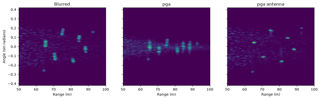
Plain pga on the blurred image makes it worse. The clutter in the out-of-beam bins dominates the estimate and the “correction” scrambles the phase. Passing pga the same antenna pattern, attitude and trajectory as the imaging operators enables the per-target weighting. shifted=False tells it the azimuth spectrum layout of an image straight from backprojection. If shift_spectrum was applied first, pass True. Unlike in plain pga the layout matters for the antenna weighting, since a wrong value mirrors the illumination weights.

def peak_db_sm(img_i):
    "Mean peak amplitude near the known targets (dB)"
    peaks = []
    for tp in targets_sm:
        i, j = target_pixel_sm(tp)
        win = img_i[max(0, i-4):i+5, max(0, j-8):j+9]
        peaks.append(20 * torch.log10(win.abs().max() + 1e-12).item())
    return np.mean(peaks)

def report_sm(name, img_i, phi_i):
    dx_i = torchbp.autofocus.phase_to_pos(phi_i, grid_sm, fc_sm, pos_sm,
                                          shifted=False)
    resid = np.std(detrend_on_track((dx_sm - dx_i).cpu().numpy(),
                                    pos_sm[:,1].cpu().numpy()))
    print(f"{name}: peak loss {peak_db_sm(img_true_sm) - peak_db_sm(img_i):.1f} dB, "
          f"position residual {1e3 * resid:.1f} mm rms")
    return dx_i

img_pga_sm, phi_pga_sm = torchbp.autofocus.pga(img_blur_sm.clone())
dx_pga_sm = report_sm("pga        ", img_pga_sm, phi_pga_sm)

img_ant_sm, phi_ant_sm = torchbp.autofocus.pga(
    img_blur_sm.clone(), grid=grid_sm, fc=fc_sm, pos=pos_sm, att=att_sm,
    g=g_sm, g_extent=g_extent_sm, shifted=False)
dx_ant_sm = report_sm("pga antenna", img_ant_sm, phi_ant_sm)

fig, axes = plt.subplots(1, 3, figsize=(15, 4), sharey=True)
show_sm(axes[0], img_blur_sm, "Blurred")
show_sm(axes[1], img_pga_sm, "pga")
show_sm(axes[2], img_ant_sm, "pga antenna")
axes[0].set_ylabel("Angle (sin radians)");

pga        : peak loss 30.2 dB, position residual 260.3 mm rms
pga antenna: peak loss 2.2 dB, position residual 15.7 mm rms

Converting the solved phases to range position errors with phase_to_pos shows the antenna weighting recovering the shape of the injected error while plain PGA diverges. The mean and linear trend are unobservable to PGA, so the comparison is detrended.

u_sm = pos_sm[:,1].cpu().numpy()

plt.figure(figsize=(8, 4))
plt.plot(u_sm, 1e3 * detrend_on_track(dx_sm.cpu().numpy(), u_sm), "k",
         label="Applied")
plt.plot(u_sm, 1e3 * detrend_on_track(dx_ant_sm.cpu().numpy(), u_sm),
         label="pga antenna")
plt.plot(u_sm, 1e3 * detrend_on_track(dx_pga_sm.cpu().numpy(), u_sm),
         label="pga")
plt.legend()
plt.xlabel("Aperture position (m)")
plt.ylabel("x error (mm)");

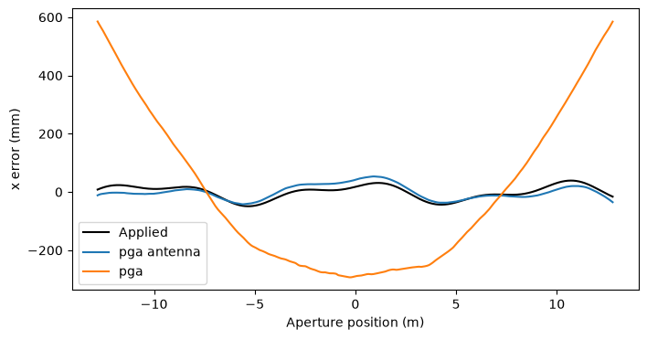
The remaining residual is not estimation noise but a limit of the method. The correction is a single phase profile applied to the whole image, while at this low altitude the elevation angle varies across the swath, so no single phase correction fits every target exactly. When the raw data is available, the pulse-domain gpga / gpga_tde with the same antenna arguments avoids that limit entirely (see the GPGA example).