Antenna pattern normalization

In SAR image the pixels are brighter where the antenna is pointed and at closer distances. This is caused by the two-way antenna gain and the free-space spreading loss, not by the scene itself. To compare reflectivities across an image the effect of antenna and distance has to be removed.

torchbp models the illumination directly with backprojection_polar_2d_tx_power. Given the antenna gain pattern, the trajectory and the antenna attitude, it forms a pseudo-polar image of the square-root power that a constant reflectivity ground would return. Dividing the SAR image by this map removes the antenna footprint and the range falloff, leaving an image whose brightness reflects the scene.

This example:

1. Creates synthetic data

2. Simulates a pass over a uniform field of random scatterers with projection_cart_2d_nufft.

3. Forms the SAR image and shows the antenna footprint imprinted on it.

4. Models the illumination with backprojection_polar_2d_tx_power and normalizes the image with it.

import torch
import numpy as np
import torchbp
import matplotlib.pyplot as plt
from numpy import hamming
import time

Use CUDA if available.

if torch.cuda.is_available():
    device = "cuda"
else:
    device = "cpu"
print("Device:", device)

Device: cpu

Radar and acquisition geometry

A small FMCW radar is flown along the \(y\) axis at 45 m altitude, looking in the \(+x\) direction. The low altitude relative to the imaged range means the elevation angle changes a lot across the swath, so the elevation antenna pattern shows up strongly as a range-dependent brightness.

fc = 6e9            # RF center frequency (Hz)
bw = 200e6          # Sweep bandwidth (Hz)
tsweep = 100e-6     # Sweep length (s)
fs = 5e6           # Sampling frequency (Hz)
nsamples = int(fs * tsweep)   # Time-domain samples per sweep
nsweeps = 384       # Number of azimuth measurements
wl = 3e8 / fc       # Wavelength

altitude = 45.0     # Platform altitude (m)
element_spacing = 0.25 * wl   # Azimuth sampling along the track

Polar imaging grid. theta is the sine of the azimuth angle. The number of range and azimuth bins is chosen from the range resolution and the synthetic aperture so the grid is slightly oversampled.

r0, r1 = 60.0, 250.0      # Ground-range extent (m)
theta_limit = 0.75         # Azimuth half-extent (sine of angle)

res = 3e8 / (2 * bw)      # Slant-range resolution
res_interp = 1.3          # Grid oversampling factor
nr = int(res_interp * (r1 - r0) / res)
ntheta = int(1 + nsweeps * res_interp * (element_spacing / wl) * theta_limit / 0.25)

grid_polar = {"r": (r0, r1), "theta": (-theta_limit, theta_limit),
              "nr": nr, "ntheta": ntheta}
print("nr:", nr, "ntheta:", ntheta, "nsamples:", nsamples)

nr: 329 ntheta: 375 nsamples: 500

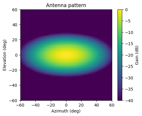
Antenna pattern

The operators take the square root of the two-way antenna gain g. If TX and RX antennas are identical, this is just the antenna pattern, but if they are not then this should be \(\sqrt{g_{tx} g_{rx}}\). It’s sampled on a regular grid of elevation x azimuth angles in radians, with the beam center at angle \((0, 0)\). The corresponding angular extent is given as g_extent = [el0, az0, el1, az1].

Here we use a separable Gaussian beam: a narrow pencil beam in elevation and a wider beam in azimuth.

naz, nel = 64, 64
az = np.linspace(-np.pi / 3, np.pi / 3, naz)
el = np.linspace(-np.pi / 3, np.pi / 3, nel)
az_bw = np.deg2rad(30)    # Azimuth beamwidth
el_bw = np.deg2rad(14)    # Elevation beamwidth

gain = np.exp(-(el[:, None] / el_bw) ** 2) * np.exp(-(az[None, :] / az_bw) ** 2)  # [el, az]
g = torch.tensor(gain, dtype=torch.float32, device=device)
g_extent = [el[0], az[0], el[-1], az[-1]]   # [el0, az0, el1, az1]

plt.figure(figsize=(5, 4))
plt.imshow(20 * np.log10(gain), origin="lower", aspect="auto",
           extent=[np.rad2deg(az[0]), np.rad2deg(az[-1]),
                   np.rad2deg(el[0]), np.rad2deg(el[-1])], vmin=-40, vmax=0)
plt.colorbar(label="Gain (dB)")
plt.xlabel("Azimuth (deg)")
plt.ylabel("Elevation (deg)")
plt.title("Antenna pattern");

Scene

To see the antenna footprint we need uniform scene: a dense field of random complex scatterers on a Cartesian grid on the ground (\(z = 0\)). Each cell has unit expected power, so any brightness variation in the SAR image comes from the illumination, not from the scene.

torch.manual_seed(0)
grid_proj = {"x": (40.0, 270.0), "y": (-270.0, 270.0), "nx": 512, "ny": 512}
img = torch.randn([grid_proj["nx"], grid_proj["ny"]], dtype=torch.complex64, device=device)

Platform trajectory and attitude

The platform flies straight along \(y\) at \(x = 0\). The antenna is rolled so the elevation beam center points at the middle of the swath; without this roll the narrow elevation beam would mostly miss the ground. The attitude att holds the [roll, pitch, yaw] Euler angles per sweep.

y_coords = torch.linspace(-nsweeps / 2, nsweeps / 2, nsweeps) * element_spacing
pos = torch.zeros([nsweeps, 3], dtype=torch.float32, device=device)
pos[:, 1] = y_coords
pos[:, 2] = altitude

r_mid = 0.5 * (r0 + r1)
roll = -np.arctan2(altitude, r_mid)   # tilt elevation beam down to mid-swath
att = torch.zeros_like(pos)
att[:, 0] = roll
print("Antenna roll:", np.rad2deg(roll), "deg")

Antenna roll: -16.189206257026942 deg

Forward projection and image formation

We simulate the raw radar data with projection_cart_2d_nufft, passing the antenna pattern (g, g_extent) and attitude (att) so that each scatterer is weighted by the two-way gain in the direction it is seen. The forward model is the point-target radar equation: amplitude \(\propto g / R^2\). After projection the raw data is range-compressed (windowed, oversampled IFFT) and backprojected onto the polar grid. The data_fmod term centers the range spectrum around DC to reduce interpolation error.

"sigma" normalization means that input scene RCS is normalized to \(1~m^2\) area.

Alternatives are:

• "beta" (normalized to slant-range area)

• "gamma" (normalized to area projected towards radar)

• "point" (point target with fixed RCS).

oversample = 2
data_fmod = -torch.pi * (1 - (oversample - 1) / oversample)
n = nsamples * oversample
r_res = 3e8 / (2 * bw * oversample)

t = time.time()
# Forward project the scene to raw FMCW data (stop-and-go NUFFT) with the antenna pattern
data = torchbp.ops.projection_cart_2d_nufft(
    img, pos, grid_proj, fc, fs, bw / tsweep, nsamples,
    att=att, g=g, g_extent=g_extent, use_rvp=False, normalization="sigma")[0]
# Range compression: window + oversampled IFFT
w = torch.tensor(hamming(data.shape[-1])[None, :], dtype=torch.float32, device=device)
data = torch.fft.ifft(data * w, dim=-1, n=n)
data = data * torch.exp(1j * data_fmod * torch.arange(data.shape[-1], device=device))[None, :]
# Backproject to the polar grid
sar = torchbp.ops.backprojection_polar_2d(
    data, grid_polar, fc, r_res, pos, dealias=False, data_fmod=data_fmod)[0]
print(f"Image formed in {time.time() - t:.2f} s")

Image formed in 2.48 s

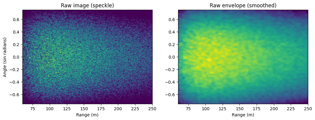
The raw image is dominated by speckle, so to see the illumination we smooth the power with a small box filter. The smoothed envelope clearly shows the antenna footprint: a bright blob centered mid-swath where the rolled pencil beam illuminates the ground, fading toward the range edges (elevation pattern + range loss) and toward the azimuth edges (azimuth pattern).

def envelope(x):
    """Smoothed magnitude (power box filter) to reveal the illumination under speckle."""
    p = (torch.abs(x) ** 2)[None, None]
    p = torch.nn.functional.avg_pool2d(p, 9, stride=1, padding=4)[0, 0]
    return torch.sqrt(p)

extent = [*grid_polar["r"], *grid_polar["theta"]]
env = envelope(sar)

fig, axes = plt.subplots(1, 2, figsize=(12, 4))
for ax, x, title in zip(axes, [sar, env], ["Raw image (speckle)", "Raw envelope (smoothed)"]):
    db = 20 * torch.log10(torch.abs(x) + 1e-12).cpu().numpy()
    m = db.max()
    im = ax.imshow(db.T, origin="lower", vmin=m - 35, vmax=m, extent=extent, aspect="auto")
    ax.set_title(title)
    ax.set_xlabel("Range (m)")
axes[0].set_ylabel("Angle (sin radians)");

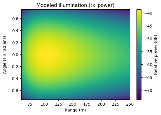
Modeling the illumination

backprojection_polar_2d_tx_power forms this from the geometry. For every polar pixel it sums the two-way gain \(g^2\) over all sweeps, weighted by the range loss, and returns the square-root power that a constant-reflectivity ground would return. Its inputs mirror the image formation:

• wa per-sweep amplitude weighting (transmit power and/or an azimuth window). Here it is flat.

• g, g_extent, att, pos, grid_polar, r_res the same antenna pattern, attitude and geometry used to form the image.

• normalization the radiometric convention. "beta" gives the raw illumination of the imaging plane. "sigma" and "gamma" additionally divide by the incidence-angle terms to estimate \(\sigma_0\) / \(\gamma_0\) backscatter coefficients. "point" normalizes for point targets.

• azimuth_resolution (default True) additionally folds in the azimuth-resolution normalization, so dividing by tx_power also flattens the residual azimuth brightness. Pass False to get the pure antenna/range illumination.

The modeled footprint matches the measured envelope above.

wa = torch.ones(nsweeps, device=device)   # flat per-sweep weighting

tx_power = torchbp.ops.backprojection_polar_2d_tx_power(
    wa, g, g_extent, grid_polar, r_res, pos, att, normalization="sigma")[0]

plt.figure(figsize=(6, 4))
db = 20 * torch.log10(tx_power + 1e-12).cpu().numpy()
m = db.max()
plt.imshow(db.T, origin="lower", vmin=m - 35, vmax=m, extent=extent, aspect="auto")
plt.colorbar(label="Relative power (dB)")
plt.xlabel("Range (m)")
plt.ylabel("Angle (sin radians)")
plt.title("Modeled illumination (tx_power)");

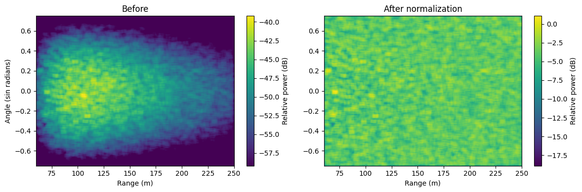
Normalization

Dividing the SAR image by the modeled illumination removes the antenna footprint and the range falloff. The residual still has speckle noise.

sar_norm = sar / tx_power
env_norm = envelope(sar_norm)

fig, axes = plt.subplots(1, 2, figsize=(12, 4))
for ax, x, title in zip(axes, [env, env_norm], ["Before", "After normalization"]):
    db = 20 * torch.log10(torch.abs(x) + 1e-12).cpu().numpy()
    m = db.max()
    im = ax.imshow(db.T, origin="lower", vmin=m - 20, vmax=m, extent=extent, aspect="auto")
    ax.set_title(title)
    ax.set_xlabel("Range (m)")
    plt.colorbar(im, ax=ax, label="Relative power (dB)")
axes[0].set_ylabel("Angle (sin radians)")
plt.tight_layout();

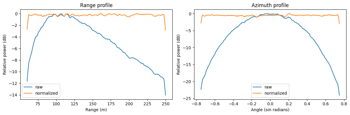
Range and azimuth profiles

r_axis = np.linspace(r0, r1, nr)
th_axis = np.linspace(-theta_limit, theta_limit, ntheta)

def db(x):
    return 20 * torch.log10(x + 1e-12).cpu().numpy()

fig, axes = plt.subplots(1, 2, figsize=(12, 4))
axes[0].plot(r_axis, db(env.mean(1)) - db(env.mean(1)).max(), label="raw")
axes[0].plot(r_axis, db(env_norm.mean(1)) - db(env_norm.mean(1)).max(), label="normalized")
axes[0].set_xlabel("Range (m)")
axes[0].set_ylabel("Relative power (dB)")
axes[0].set_title("Range profile")
axes[0].legend()

axes[1].plot(th_axis, db(env.mean(0)) - db(env.mean(0)).max(), label="raw")
axes[1].plot(th_axis, db(env_norm.mean(0)) - db(env_norm.mean(0)).max(), label="normalized")
axes[1].set_xlabel("Angle (sin radians)")
axes[1].set_ylabel("Relative power (dB)")
axes[1].set_title("Azimuth profile")
axes[1].legend()
plt.tight_layout();

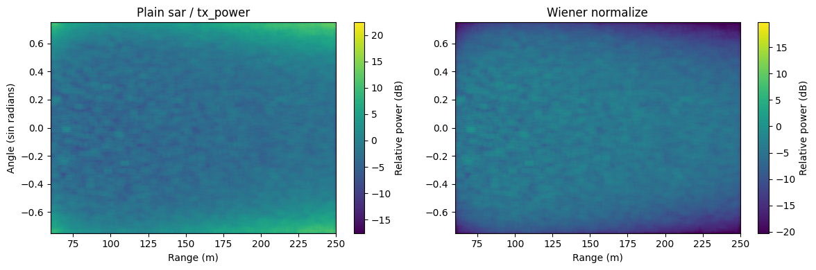
SNR-aware normalization

With real data the illumination is poor at the swath edges and antenna nulls. There tx_power is tiny, and dividing the SAR image by it divides receiver noise by an almost-zero number, so the normalized edges explode with amplified noise.

torchbp.util.wiener_normalize replaces the division by the Wiener (MMSE) estimate

\[\hat{s} = \frac{\mathrm{sar}\cdot\mathrm{tx\_power}}{\mathrm{tx\_power}^2 + \varepsilon^2} = \frac{\mathrm{sar}}{\mathrm{tx\_power}}\cdot\frac{\mathrm{SNR}}{1+\mathrm{SNR}}, \qquad \mathrm{SNR} = \left(\frac{\mathrm{tx\_power}}{\varepsilon}\right)^2.\]

Where the illumination is strong this is the full normalization; where it is weak the gain rolls off as \(\mathrm{tx\_power}^2\), so the output goes to zero instead of blowing up.

The regularization \(\varepsilon = \sigma_n/\sigma_s\) is the noise-to-signal amplitude ratio in tx_power units, the illumination level where the SNR is one. It isn’t simply the noise level \(\sigma_n\): with the model \(\mathrm{sar} = s\cdot\mathrm{tx\_power} + n\) the noise amplitude \(\sigma_n\) must be divided by the reflectivity scale \(\sigma_s\), which also absorbs the leftover radiometric calibration constant of tx_power. When eps is not given it is estimated from the data using \(E|\mathrm{sar}|^2 = \sigma_s^2\,\mathrm{tx\_power}^2 + \sigma_n^2\): \(\sigma_s^2\) from the brightest pixels and \(\sigma_n^2\) from the dimmest. For real data prefer an explicit value from a shadow region and a calibration target.

To show the effect we add receiver noise to the SAR image (constant noise, but the signal fades toward the edges) and compare plain division with the Wiener estimate.

# Emulate receiver noise constant complex noise added to the SAR image.
torch.manual_seed(1)
noise_std = 0.5 * sar.abs().mean() # sigma_n: noise amplitude
sar_noisy = sar + noise_std * torch.randn_like(sar)

# The correct regularization is eps = sigma_n / sigma_s, the noise-to-signal ratio
# in tx_power units. sigma_s is the reflectivity scale relating
# the image to the illumination (sar = s * tx_power + n), it also absorbs the
# leftover calibration constant of tx_power. Measure it where illumination is strong.
bright = tx_power > tx_power.quantile(0.8)
sigma_s = ((sar / tx_power).abs()[bright] ** 2).mean().sqrt()
eps = noise_std / sigma_s
print(f"sigma_n = {float(noise_std):.2e}, sigma_s = {float(sigma_s):.3f}, eps = {float(eps):.2e}")

naive = sar_noisy / tx_power
wiener = torchbp.util.wiener_normalize(sar_noisy, tx_power, eps=eps)
# Passing eps=None makes wiener_normalize estimate the same value from the data.

fig, axes = plt.subplots(1, 2, figsize=(12, 4))
for ax, x, title in zip(axes, [naive, wiener], ["Plain sar / tx_power", "Wiener normalize"]):
    d = 20 * torch.log10(envelope(x) + 1e-12).cpu().numpy()
    m = np.nanmedian(d)
    im = ax.imshow(d.T, origin="lower", vmin=m - 15, vmax=m + 25, extent=extent, aspect="auto")
    ax.set_title(title)
    ax.set_xlabel("Range (m)")
    plt.colorbar(im, ax=ax, label="Relative power (dB)")
axes[0].set_ylabel("Angle (sin radians)")
plt.tight_layout();

sigma_n = 1.20e-03, sigma_s = 0.643, eps = 1.87e-03

The calibration is still missing a constant factor. If calibrated RCS values are needed this constant factor needs to be also solved. It can be found by imaging a known RCS target, usually a corner reflector.

For slant-range images (BP origin at sensor altitude, pos z = 0) use backprojection_polar_2d_tx_power_slant, which takes the sensor altitude and maps each polar pixel to its ground position before computing angles.