Backprojection image formation
[1]:
import torch
import torchbp
import matplotlib.pyplot as plt
from numpy import hamming
Use CUDA if available
[2]:
if torch.cuda.is_available():
    device = "cuda"
else:
    device = "cpu"
print("Device:", device)
Device: cpu
Constant definitions
[3]:
nr = 128 # Range points
ntheta = 128 # Azimuth points
nsweeps = 128 # Number of measurements
fc = 6e9 # RF center frequency
bw = 100e6 # RF bandwidth. Negative for falling sweep.
tsweep = 100e-6 # Sweep length
fs = 1e6 # Sampling frequency
nsamples = int(fs * tsweep) # Time domain samples per sweep

# Imaging grid definition. Azimuth angle "theta" is sine of radians. 0.2 = 11.5 degrees.
grid_polar = {"r": (90, 110), "theta": (-0.2, 0.2), "nr": nr, "ntheta": ntheta}
Define target and radar positions. There is one point target at 100 m distance and zero azimuth angle. For polar image formation radar motion should be in direction of Y-axis. If this is not the case positions should be rotated.
[4]:
target_pos = torch.tensor([[100, 0, 0]], dtype=torch.float32, device=device)
target_rcs = torch.tensor([[1]], dtype=torch.float32, device=device)
pos = torch.zeros([nsweeps, 3], dtype=torch.float32, device=device)
pos[:,1] = torch.linspace(-nsweeps/2, nsweeps/2, nsweeps) * 0.25 * 3e8 / fc
pos[:,2] = 50 # Platform height
Generate synthetic radar data
[5]:
# Oversampling input data decreases interpolation errors
oversample = 2
# Modulation frequency in range direction to center the spectrum at DC
# for more accurate interpolation.
data_fmod = -torch.pi * (1 - (oversample-1) / oversample)
print("data_fmod", data_fmod)
data = torchbp.util.generate_fmcw_data(target_pos, target_rcs, pos, fc, bw, tsweep, fs)
# Apply windowing function in range direction
w = torch.tensor(hamming(data.shape[-1])[None,:], dtype=torch.float32, device=device)
# With rising sweep the IF frequencies are negative.
if bw > 0:
data = torch.fft.ifft(data * w, dim=-1, n=nsamples * oversample)
else:
data = torch.fft.ifft(data.conj() * w, dim=-1, n=nsamples * oversample).conj()
data_fmod = -data_fmod
data_fmod_f = torch.exp(1j*data_fmod*torch.arange(data.shape[-1], device=device))[None,:]
data = data * data_fmod_f
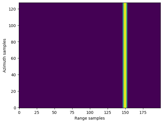
data_db = 20*torch.log10(torch.abs(data)).detach()
m = torch.max(data_db)
plt.figure()
plt.imshow(data_db.cpu().numpy(), origin="lower", vmin=m-30, vmax=m, aspect="auto")
plt.xlabel("Range samples")
plt.ylabel("Azimuth samples");
data_fmod -1.5707963267948966
Plot the range spectrum of the raw data. With correct data_fmod, the spectrum should be centered around 0.
[6]:
freqs = torch.fft.fftshift(torch.fft.fftfreq(data.shape[-1]))
plt.figure()
plt.plot(freqs.cpu().numpy(), 20*torch.log10(torch.abs(torch.fft.fftshift(torch.fft.fft(data[0])))).cpu().numpy())
plt.xlabel("Frequency (cycles/sample)")
plt.ylabel("Magnitude (dB)");
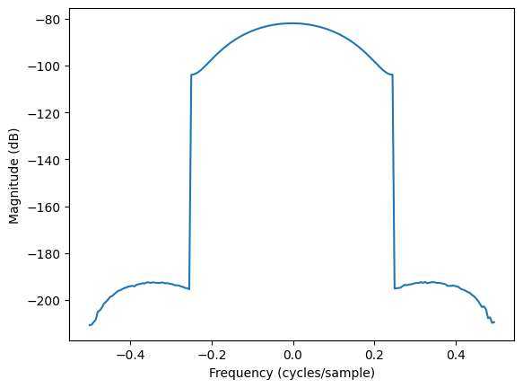
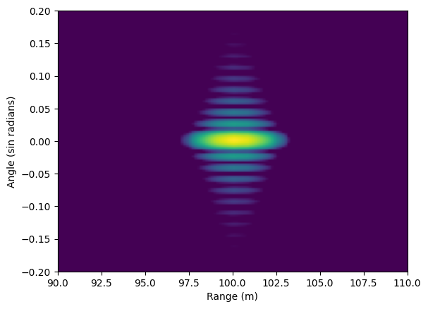
Image formation. Hamming window was applied in range direction so low sidelobes in range are expected. Azimuth direction has no windowing function and high sidelobes (Highest -13 dB) are expected. Azimuth sidelobes could be decreased by windowing the input data also in the other dimension.
[7]:
r_res = 3e8 / (2 * abs(bw) * oversample) # Range bin size in input data

# Calculate modulation frequency to center the spectrum of image around DC for decreased interpolation error.
dr = (grid_polar["r"][1] - grid_polar["r"][0]) / grid_polar["nr"]
im_margin = oversample * r_res / dr - 1
alias_fmod = -torch.pi * (1 - im_margin / (1 + im_margin))
if bw < 0:
    alias_fmod = -alias_fmod

img = torchbp.ops.backprojection_polar_2d(data, grid_polar, fc, r_res, pos, dealias=True, data_fmod=data_fmod, alias_fmod=alias_fmod)
img = img.squeeze() # Removes singular batch dimension

img_db = 20*torch.log10(torch.abs(img)).detach()

m = torch.max(img_db)

extent = [*grid_polar["r"], *grid_polar["theta"]]

plt.figure()
plt.imshow(img_db.cpu().numpy().T, origin="lower", vmin=m-30, vmax=m, extent=extent, aspect="auto")
plt.xlabel("Range (m)")
plt.ylabel("Angle (sin radians)");
Plot the SAR image spectrum. It should be centered around 0,0 with correct alias_fmod choice.
[8]:
plt.figure()
fimg = torch.fft.fftshift(torch.fft.fft2(img), (0, 1))
fimg_db = (20*torch.log10(torch.abs(fimg)))
vmax = torch.max(fimg_db)
plt.imshow(fimg_db.cpu().numpy(), origin="lower", aspect="auto", vmin=vmax-40, vmax=vmax, extent=[-0.5, 0.5, -0.5, 0.5])
plt.xlabel("Cross-range frequency (cycles/sample)")
plt.ylabel("Range frequency (cycles/sample)");
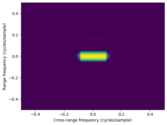
Image entropy. Can be used as a loss function for optimization.
[9]:
entropy = torchbp.util.entropy(img)
print("Entropy:", entropy.item())
Entropy: 7.45965576171875
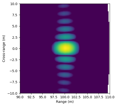
Convert image to cartesian coordinates:
[10]:
# Origin of the polar coordinates
origin = torch.mean(pos, axis=0)
# Cartesian grid definition
grid_cart = {"x": (90, 110), "y": (-10, 10), "nx": 128, "ny": 128}

img_cart = torchbp.ops.polar_to_cart(img, origin, grid_polar, grid_cart, fc, rotation=0, alias_fmod=alias_fmod, method=("lanczos", 10))

img_db = 20*torch.log10(torch.abs(img_cart)).detach()

m = torch.max(img_db)

extent = [*grid_cart["x"], *grid_cart["y"]]

plt.figure()
plt.imshow(img_db.cpu().numpy().T, origin="lower", vmin=m-30, vmax=m, extent=extent, aspect="equal")
plt.xlabel("Range (m)")
plt.ylabel("Cross-range (m)");
Backprojection directly onto Cartesian grid
[11]:
img_cart2 = torchbp.ops.backprojection_cart_2d(data, grid_cart, fc, r_res, pos, data_fmod=data_fmod)
img_cart2 = img_cart2.squeeze() # Removes singular batch dimension

img_db = 20*torch.log10(torch.abs(img_cart2)).detach()

m = torch.max(img_db)

extent = [*grid_cart["x"], *grid_cart["y"]]

plt.figure()
plt.imshow(img_db.cpu().numpy().T, origin="lower", vmin=m-30, vmax=m, extent=extent, aspect="equal")
plt.xlabel("Range (m)")
plt.ylabel("Cross-range (m)");
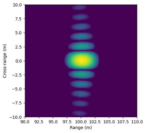
Difference between the results should be very small
[12]:
plt.figure()
plt.title("Phase difference")
plt.imshow(torch.angle(img_cart * torch.conj(img_cart2)).cpu().numpy().T, origin="lower", extent=extent, aspect="equal")
plt.xlabel("Range (m)")
plt.ylabel("Cross-range (m)");
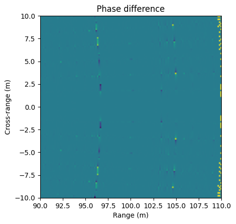
[13]:
torch.linalg.norm(img_cart - img_cart2) / torch.linalg.norm(img_cart)
[13]:
tensor(0.0020)
[ ]: