Backprojection on DEM

Backprojection normally assumes that every image pixel lies on the \(z = 0\) plane. A scatterer at height above the zero-height plane has a shorter slant range than a flat ground point at the same image coordinates, so on a flat-earth image it lands displaced towards the radar (layover). The displacement grows with target height and with the look angle, and since it varies across the scene with the terrain the image gets warped.

backprojection_polar_2d and ffbp take an optional dem argument that replaces the flat-earth assumption with per-pixel terrain heights:

• dem is a float32 tensor of shape [dem_nr, dem_ntheta] covering the same r/theta extent as the image grid. It can be much coarser than the image grid, heights are bilinearly interpolated at each pixel.

• Values are pixel z coordinates in the same frame as the platform positions.

• DEM sample [i, j] corresponds to image pixel (i * nr / dem_nr,   j * ntheta / dem_ntheta). Sample i sits at r0 + i * (r1 - r0) / dem_nr.

• torchbp.util.dem_to_polar resamples a real Cartesian DEM (e.g. from a GeoTIFF) to a polar grid. In this example a synthetic DEM is built directly.

This notebook builds a synthetic terrain with a grid of point targets on it, and shows that with the DEM the targets focus at their correct image coordinates while the flat-earth image misplaces them.

import math
import torch
import numpy as np
import matplotlib.pyplot as plt
from numpy import hamming

import torchbp
from torchbp.ops import backprojection_polar_2d, ffbp

device = "cuda" if torch.cuda.is_available() else "cpu"
print("Device:", device)

Device: cpu

Scene: terrain and a grid of point targets

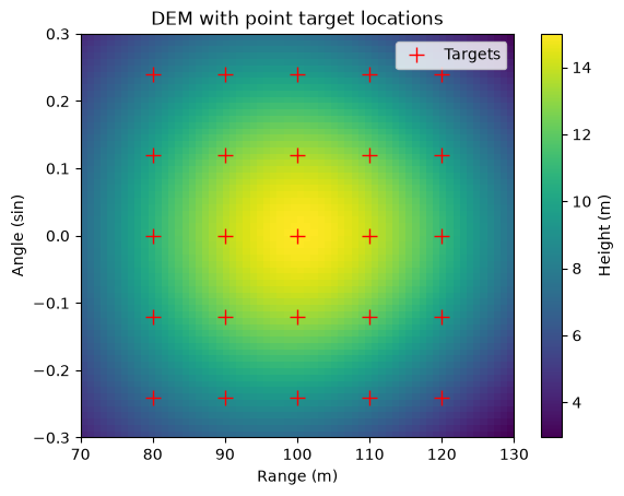
The terrain is a smooth 15 m high hill in the middle of the scene. A 5x5 grid of equal point targets is placed on the terrain surface, so targets near the scene center are elevated and the ones at the edges are close to the ground plane. The platform flies a straight track along y at 50 m height, so the look angle is fairly steep and the layover displacement is several meters at the hilltop.

fc = 6e9          # RF center frequency (Hz)
bw = 200e6        # RF bandwidth (Hz)
tsweep = 100e-6   # Sweep length (s)
fs = 2e6          # Sampling frequency (Hz)
nsweeps = 512     # Number of pulses in the aperture
oversample = 2    # Range FFT oversampling
nsamples = int(fs * tsweep)

nr, ntheta = 320, 384
grid = {"r": (70.0, 130.0), "theta": (-0.3, 0.3), "nr": nr, "ntheta": ntheta}
r0, r1 = grid["r"]
t0, t1 = grid["theta"]

def terrain(x, y):
    """Terrain height (m) as a function of world x, y."""
    return 15.0 * torch.exp(-((x - 100.0)**2 + y**2) / (2 * 25.0**2))

# 5x5 grid of point targets on the terrain surface.
rt = torch.linspace(80.0, 120.0, 5)
tt = torch.linspace(-0.24, 0.24, 5)
R, T = torch.meshgrid(rt, tt, indexing="ij")
xt = (R * torch.sqrt(1 - T**2)).flatten()
yt = (R * T).flatten()
zt = terrain(xt, yt)
target_pos = torch.stack([xt, yt, zt], dim=1).to(torch.float32).to(device)
target_rcs = torch.ones((target_pos.shape[0], 1), dtype=torch.float32, device=device)

# Straight track along y at 50 m height, lambda/4 element spacing.
pos = torch.zeros((nsweeps, 3), dtype=torch.float32, device=device)
pos[:, 1] = torch.linspace(-nsweeps / 2, nsweeps / 2, nsweeps, device=device) * 0.25 * 3e8 / fc
pos[:, 2] = 50.0

Synthetic DEM on the polar grid

The DEM is sampled at 64x64 points, much coarser than the 320x384 image grid, to demonstrate that the kernel’s bilinear interpolation handles the resolution difference. Sample [i, j] is placed at the cell-start coordinates r = r0 + i*(r1-r0)/dem_nr, theta = t0 + j*(t1-t0)/dem_ntheta to match the kernel’s pixel-to-DEM index map.

dem_nr, dem_ntheta = 64, 64
r_dem = r0 + (r1 - r0) * torch.arange(dem_nr, device=device) / dem_nr
t_dem = t0 + (t1 - t0) * torch.arange(dem_ntheta, device=device) / dem_ntheta
x_dem = r_dem[:, None] * torch.sqrt(1 - t_dem[None, :]**2)
y_dem = r_dem[:, None] * t_dem[None, :]
dem = terrain(x_dem, y_dem).to(torch.float32)

plt.figure()
plt.imshow(dem.cpu().numpy().T, origin="lower", extent=[r0, r1, t0, t1], aspect="auto")
plt.colorbar(label="Height (m)")
plt.plot((xt**2 + yt**2).sqrt().cpu(), (yt / (xt**2 + yt**2).sqrt()).cpu(), "r+", ms=10, label="Targets")
plt.xlabel("Range (m)")
plt.ylabel("Angle (sin)")
plt.title("DEM with point target locations")
plt.legend(loc="best")
plt.show()

Simulate and range-compress the data

generate_fmcw_data uses the true 3D target positions, so the raw data contains the real terrain geometry. Range window, FFT range compression, and the data_fmod spectrum shift that reduces interpolation error.

raw = torchbp.util.generate_fmcw_data(target_pos, target_rcs, pos, fc, bw, tsweep, fs)
w = torch.tensor(hamming(raw.shape[-1])[None, :], dtype=torch.float32, device=device)
data = torch.fft.ifft(raw * w, dim=-1, n=nsamples * oversample)

data_fmod = -math.pi * (1 - (oversample - 1) / oversample)
data = data * torch.exp(1j * data_fmod * torch.arange(data.shape[-1], device=device))[None, :]

r_res = 3e8 / (2 * abs(bw) * oversample)
dr = (grid["r"][1] - grid["r"][0]) / grid["nr"]
im_margin = oversample * r_res / dr - 1
alias_fmod = -math.pi * (1 - im_margin / (1 + im_margin))
print(f"r_res = {r_res:.3f} m, image dr = {dr:.3f} m")

r_res = 0.375 m, image dr = 0.188 m

extent = [r0, r1, t0, t1]

def show_polar(img, title, ax=None, dyn=35, ref_max=None):
    img = img.detach().cpu()
    db = 20 * torch.log10(torch.abs(img) + 1e-12)
    m = db.max() if ref_max is None else ref_max
    if ax is None:
        _, ax = plt.subplots()
    ax.imshow(db.numpy().T, origin="lower", vmin=m - dyn, vmax=m,
              extent=extent, aspect="auto")
    # True target positions in image coordinates.
    r_t = (xt**2 + yt**2).sqrt().cpu()
    ax.plot(r_t, (yt.cpu() / r_t), "o", ms=10, mfc="none", mec="r", label="True position")
    ax.set_title(title)
    ax.set_xlabel("Range (m)")
    ax.set_ylabel("Angle (sin)")
    ax.legend(loc="upper right")
    return m

Image with and without the DEM

Both images are formed with ffbp from the same data, the only difference is the dem argument. The red circles mark the true target coordinates.

img_flat = ffbp(data, grid, fc, r_res, pos, stages=4, dealias=True,
                data_fmod=data_fmod, alias_fmod=alias_fmod).squeeze()
img_dem = ffbp(data, grid, fc, r_res, pos, stages=4, dealias=True,
               data_fmod=data_fmod, alias_fmod=alias_fmod, dem=dem).squeeze()

fig, axs = plt.subplots(1, 2, figsize=(12, 4.5))
m = show_polar(img_flat, "FFBP, flat earth", ax=axs[0])
show_polar(img_dem, "FFBP with DEM", ax=axs[1], ref_max=m)
plt.tight_layout()
plt.show()

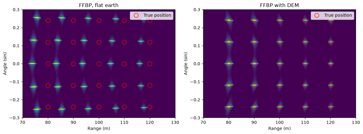
Without the DEM every elevated target is displaced towards the radar. The higher the terrain under it, the larger the shift, so the regular target grid appears warped around the hill. The near-ground targets at the scene edges sit close to their circles in both images. With the DEM all 25 targets focus on their true coordinates.

For a straight track the flat-earth error is almost purely a position error and the point-spread functions stay compact, they are just at wrong places.

FFBP against direct backprojection

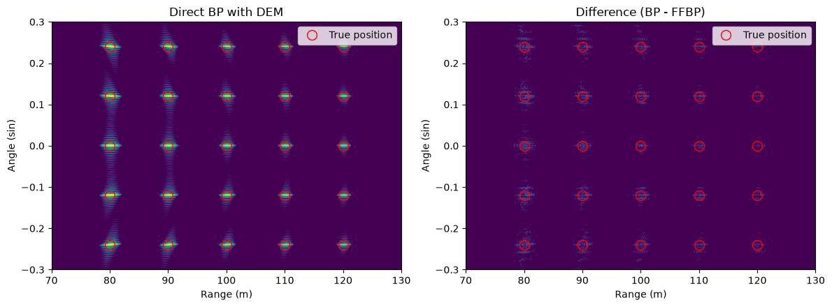
The DEM-aware FFBP merge should match direct backprojection on the same DEM. With a DEM the dealias carrier is always referenced to the DEM surface instead of the z=0 plane: a flat-plane carrier would leave a terrain-dependent residual phase that aliases the image spectrum on any significant topography, defeating the purpose of dealiasing. torchbp.util.bp_polar_range_dealias and bp_polar_range_alias take the same dem argument to apply or remove this carrier after image formation. These functions could be required for example with interferometric SAR processing.

img_bp_dem = backprojection_polar_2d(data, grid, fc, r_res, pos, dealias=True,
                                     data_fmod=data_fmod, alias_fmod=alias_fmod,
                                     dem=dem).squeeze()

def relerr(a, b):
    return (torch.linalg.norm(a - b) / torch.linalg.norm(a)).item()

print(f"FFBP+DEM vs direct BP+DEM relative error: {relerr(img_bp_dem, img_dem):.4f}")

fig, axs = plt.subplots(1, 2, figsize=(12, 4.5))
show_polar(img_bp_dem, "Direct BP with DEM", ax=axs[0], ref_max=m)
show_polar(img_bp_dem - img_dem, "Difference (BP - FFBP)", ax=axs[1], ref_max=m, dyn=60)
plt.tight_layout()
plt.show()

FFBP+DEM vs direct BP+DEM relative error: 0.0121

Notes

• With real measurement data, resample the DEM onto the polar grid with torchbp.util.dem_to_polar and make sure its heights are in the same z frame as the platform positions.

• The autofocus functions torchbp.autofocus.gpga and gpga_tde also accept dem.