Interferometry with synthetic data

Synthetic Aperture Radar interferometry (InSAR) recovers terrain height by comparing the phases of two SAR images acquired from slightly different positions. The phase difference between the two images (interferogram) depends on the path-length difference from each antenna to the ground, which depends on the local terrain height and the baseline separation of the two acquisitions.

This example:

1. Builds a synthetic scene of random scatterers on top of a smooth digital elevation model (DEM).

2. Simulates two FMCW radar passes with a small vertical baseline using forward projection operator in torchbp.

3. Forms SAR images of both passes and computes their interferogram.

4. Compares the measured interferogram against an analytic prediction derived directly from the known geometry.

A complete InSAR processing chain would then unwrap the interferometricphase (which is only known modulo \(2\pi\)) and convert it to height. torchbpdoes not include a phase-unwrapping algorithm. An external tool such as SNAPHU can be used for that step.

import torch
import numpy as np
import torch.nn.functional as F
import torchbp
import torchbp.interferometry as ti
import matplotlib.pyplot as plt
from numpy import hamming
import time

Use CUDA if available.

if torch.cuda.is_available():
    device = "cuda"
else:
    device = "cpu"
print("Device:", device)

Device: cpu

Radar and acquisition geometry

We model a small FMCW radar flown along the \(y\) axis at 100 m altitude. The two passes are separated by a 1 m vertical baseline (the second pass flies 1 m higher). The platform looks in the \(+x\) direction.

fc = 6e9            # RF center frequency (Hz)
bw = 200e6          # Sweep bandwidth (Hz)
tsweep = 100e-6     # Sweep length (s)
fs = 20e6           # Sampling frequency (Hz)
nsamples = int(fs * tsweep)   # Time-domain samples per sweep
nsweeps = 384       # Number of azimuth measurements (array elements)
wl = 3e8 / fc       # Wavelength

altitude = 100.0    # Platform altitude (m)
baseline_z = 1.0    # Vertical baseline between the two passes (m)
element_spacing = 0.25 * wl   # Azimuth sampling along the track

Polar imaging grid. theta is the sine of the azimuth angle. The number of range and azimuth bins is chosen from the range resolution and the synthetic aperture so the grid is slightly oversampled.

r0, r1 = 100.0, 250.0     # Ground-range extent (m)
theta_limit = 0.4         # Azimuth half-extent (sine of angle)

res = 3e8 / (2 * bw)      # Slant-range resolution
res_interp = 1.3          # Grid oversampling factor
nr = int(res_interp * (r1 - r0) / res)
ntheta = int(1 + nsweeps * res_interp * (element_spacing / wl) * theta_limit / 0.25)

grid_polar = {"r": (r0, r1), "theta": (-theta_limit, theta_limit),
              "nr": nr, "ntheta": ntheta}
print("nr:", nr, "ntheta:", ntheta, "nsamples:", nsamples)

nr: 260 ntheta: 200 nsamples: 2000

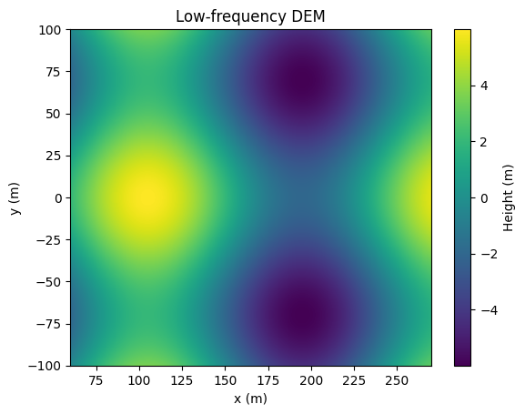
Scene

Random scatterers over a smooth DEM. The scene is defined on a Cartesian grid on the ground (\(z=0\)) plane. Each grid cell is a scatterer with a random complex amplitude. Each scatterer’s Z-coordinate is sampled from DEM so that they are at slightly different elevations. Because the DEM is smooth, the terrain height changes slowly across the scene and produces the gently curving interferometric fringes.

torch.manual_seed(0)

grid_proj = {"x": (60.0, 270.0), "y": (-100.0, 100.0), "nx": 384, "ny": 384}

# Random complex amplitude per scatterer
img = torch.randn([grid_proj["nx"], grid_proj["ny"]], dtype=torch.complex64, device=device)

# Smooth, low-frequency DEM (height in metres)
xg = torch.linspace(grid_proj["x"][0], grid_proj["x"][1], grid_proj["nx"], device=device)
yg = torch.linspace(grid_proj["y"][0], grid_proj["y"][1], grid_proj["ny"], device=device)
X, Y = torch.meshgrid(xg, yg, indexing="ij")
dem = (4.0 * torch.sin(2 * np.pi * (X - grid_proj["x"][0]) / 180.0)
       + 2.0 * torch.cos(2 * np.pi * Y / 140.0)).to(torch.float32)

extent_proj = [*grid_proj["x"], *grid_proj["y"]]
plt.figure()
plt.imshow(dem.cpu().numpy().T, origin="lower", extent=extent_proj, aspect="auto")
plt.colorbar(label="Height (m)")
plt.xlabel("x (m)")
plt.ylabel("y (m)")
plt.title("Low-frequency DEM");

Platform trajectories

Both passes fly straight along \(y\) at \(x=0\). The only difference is altitude, the second pass is baseline_z metres higher. Because both tracks share the same horizontal position, the two SAR images land on the same polar grid and no coregistration is needed. In practice the images would need to be coregistered since interferometry is very sensitive to position errors.

y_coords = torch.linspace(-nsweeps / 2, nsweeps / 2, nsweeps) * element_spacing
pos0 = torch.zeros([nsweeps, 3], dtype=torch.float32, device=device)
pos0[:, 1] = y_coords
pos0[:, 2] = altitude

pos1 = pos0.clone()
pos1[:, 2] = altitude + baseline_z

# Mean antenna phase-centre of each pass (the imaging origin)
origin0 = pos0.mean(0)
origin1 = pos1.mean(0)

Forward projection and image formation

We simulate the raw radar data with projection_cart_2d_nufft, which generates radar measurement data from the scene using non-uniform FFT. There are two forward projectors in torchbp: projection_cart_2d_nufft is fast but uses the stop-and-go approximation, the platform is assumed to be stationary during each sweep. This is accurate for typical geometries and is what we use here. projection_cart_2d is a direct evaluation that also supports intra-sweep motion (vel). It is more general but much slower (typically about 10 to 100 times).

After projection, the raw data is range-compressed (FFT with oversampling) and backprojected onto the polar grid. The data_fmod term centers the range spectrum around DC to minimize interpolation error. We backproject with dealias=False to not lose the interferometric phase (see torchbp.util.bp_polar_range_dealias for more info). Both passes are imaged on the same flat\(z=0\) grid. Note that unlike slant range image formation, flat-plane backprojection interferogram does not include flat earth phase.

oversample = 2
data_fmod = -torch.pi * (1 - (oversample - 1) / oversample)
n = nsamples * oversample
r_res = 3e8 / (2 * bw * oversample)

def make_image(pos):
    # Forward project the scene to raw FMCW data (stop-and-go NUFFT)
    data = torchbp.ops.projection_cart_2d_nufft(
        img, pos, grid_proj, fc, fs, bw / tsweep, nsamples,
        dem=dem, use_rvp=False, normalization="gamma")[0]
    # Range compression: window + oversampled IFFT
    w = torch.tensor(hamming(data.shape[-1])[None, :], dtype=torch.float32, device=device)
    data = torch.fft.ifft(data * w, dim=-1, n=n)
    data = data * torch.exp(1j * data_fmod * torch.arange(data.shape[-1], device=device))[None, :]
    # Backproject to the polar grid using FFBP, referenced to the flat z=0 plane
    return torchbp.ops.backprojection_polar_2d(
        data, grid_polar, fc, r_res, pos, dealias=False, data_fmod=data_fmod)[0]

t = time.time()
sar0 = make_image(pos0)
sar1 = make_image(pos1)
print(f"Both passes formed in {time.time() - t:.2f} s")

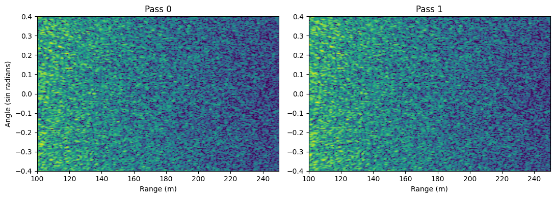
Both passes formed in 2.37 s

The two SAR images look essentially identical in magnitude. The height information is hidden in their relative phase.

extent = [*grid_polar["r"], *grid_polar["theta"]]
fig, axes = plt.subplots(1, 2, figsize=(11, 4))
for ax, sar, title in zip(axes, [sar0, sar1], ["Pass 0", "Pass 1"]):
    db = 20 * torch.log10(torch.abs(sar) + 1e-9).cpu().numpy()
    m = db.max()
    ax.imshow(db.T, origin="lower", vmin=m - 30, vmax=m, extent=extent, aspect="auto")
    ax.set_title(title)
    ax.set_xlabel("Range (m)")
axes[0].set_ylabel("Angle (sin radians)")
plt.tight_layout();

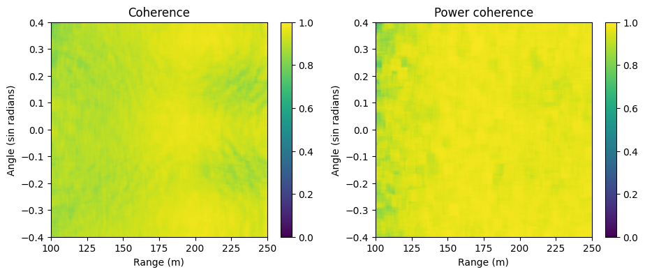
Coherence of the images calcules how well the match to each other around a small patch. Coherence of 1 means they are identical, 0 means there is no correlation. Although simulation is ideal torchbp.ops.coherence.coherence_2d is not 1 everywhere because of the DEM causes phase difference in images. For proper coherence calculation DEM phase should be removed first.

There’s also torchbp.ops.coherence.power_coherence_2d that calculates coherence without phase and is not sensitive to DEM. However, because it doesn’t use the phase it’s lower quality.

fig, axes = plt.subplots(1, 2, figsize=(11, 4))

im0 = axes[0].imshow(torchbp.ops.coherence.coherence_2d(sar0, sar1, (5,5)).cpu().numpy().T, vmin=0, vmax=1, origin="lower", aspect="auto", extent=extent)
axes[0].set_xlabel("Range (m)")
axes[0].set_ylabel("Angle (sin radians)")
axes[0].set_title("Coherence")
plt.colorbar(im0, ax=axes[0])

im1 = axes[1].imshow(torchbp.ops.coherence.power_coherence_2d(sar0, sar1, (5,5)).cpu().numpy().T, vmin=0, vmax=1, origin="lower", aspect="auto", extent=extent)
axes[1].set_xlabel("Range (m)")
axes[1].set_ylabel("Angle (sin radians)")
axes[1].set_title("Power coherence");
plt.colorbar(im0, ax=axes[1]);

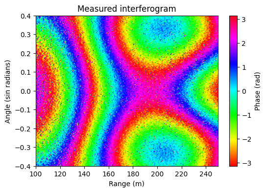
Interferogram

The interferogram is the product \(s_0 \, s_1^{*}\). Because the images were backprojected onto the flat \(z=0\) plane, the flat-earth component is already removed. The interferometric phase is topographic and, to first order, proportional to terrain height. The fringes follow the shape of the DEM.

inf = sar0 * sar1.conj()
inf_phase = torch.angle(inf).cpu().numpy()

plt.figure(figsize=(6, 4))
plt.imshow(inf_phase.T, origin="lower", cmap="hsv", extent=extent, aspect="auto")
plt.colorbar(label="Phase (rad)")
plt.xlabel("Range (m)")
plt.ylabel("Angle (sin radians)")
plt.title("Measured interferogram");

Phase unwrapping and DEM generation (not included)

The interferometric phase above is wrapped, it is only known modulo \(2\pi\). Turning it into absolute height requires phase unwrapping, which is a separate, non-trivial step.torchbp does not provide a phase-unwrapping algorithm. In a full pipeline you would export the wrapped interferogram (and a coherence map) to a dedicated unwrapper such as SNAPHU, then convert the unwrapped phase to height. For the conversion torchbp has torchbp.interferometry.phase_to_elevation_polar, which divides the unwrapped phase by the local height sensitivity\(\tfrac{4\pi}{\lambda}(z_2/r_2 - z_1/r_1)\).

Analytic interferogram

Because the geometry and DEM are known exactly, we can predict the interferogram directly.

r_arr = torch.linspace(r0, r1, nr, device=device)
theta_arr = torch.linspace(-theta_limit, theta_limit, ntheta, device=device)
# pixel x, y ground coordinates
x_w = r_arr[:, None] * torch.sqrt(1 - theta_arr[None, :] ** 2)
y_w = r_arr[:, None] * theta_arr[None, :]
r_ground = r_arr[:, None].expand_as(x_w)

def dem_at(xq, yq):
    xn = 2 * (xq - grid_proj["x"][0]) / (grid_proj["x"][1] - grid_proj["x"][0]) - 1
    yn = 2 * (yq - grid_proj["y"][0]) / (grid_proj["y"][1] - grid_proj["y"][0]) - 1
    gc = torch.stack([yn, xn], dim=-1)[None]
    return F.grid_sample(dem[None, None], gc, mode="bilinear", align_corners=True)[0, 0]

R0 = torch.sqrt(r_ground ** 2 + altitude ** 2)
# Solve for the scatterer's range in slave image.
# Layover/foreshortening shifts it in ground range.
rho = r_ground.clone()
for _ in range(6):
    s = rho / r_ground # radial scale toward the true position
    hs = dem_at(s * x_w, s * y_w)
    rho = torch.sqrt(torch.clamp(R0 ** 2 - (altitude - hs) ** 2, min=0))
R1 = torch.sqrt(rho ** 2 + (altitude + baseline_z - hs) ** 2)

phase_full = (4 * np.pi / wl) * (R1 - R0) # total geometric phase
phase_flat = (4 * np.pi / wl) * (torch.sqrt(r_ground ** 2 + (altitude + baseline_z) ** 2) - R0) # flat earth
analytic = phase_full - phase_flat # topographic phase
analytic_wrapped = torch.angle(torch.exp(1j * analytic))

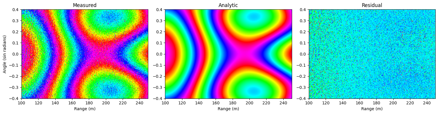
Comparison

The measured and analytic interferograms show the same topographic fringe pattern. After flattening with the analytic phase, the residual has still slight error due to layover. For more accurate DEM generation the images should be formed on a DEM. If no DEM exists, then first pass can be made without DEM and then the solved DEM is used for second pass.

diff = inf_phase - analytic.cpu().numpy()
residual = np.angle(np.exp(1j * diff))

fig, axes = plt.subplots(1, 3, figsize=(15, 4))
axes[0].imshow(inf_phase.T, origin="lower", cmap="hsv", extent=extent, aspect="auto")
axes[0].set_title("Measured")
axes[1].imshow(analytic_wrapped.cpu().numpy().T, origin="lower", cmap="hsv", extent=extent, aspect="auto")
axes[1].set_title("Analytic")
im = axes[2].imshow(residual.T, origin="lower", cmap="hsv", vmin=-np.pi, vmax=np.pi,
                    extent=extent, aspect="auto")
axes[2].set_title("Residual")
for ax in axes:
    ax.set_xlabel("Range (m)")
axes[0].set_ylabel("Angle (sin radians)")
plt.tight_layout();

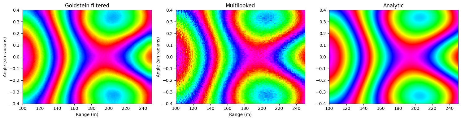
Speckle makes the interferogram noisy. It can filtered with multilooking (spatial averaging) or Goldstein phase filter. Both trade resolution for less speckle noise.

inf_gold = torchbp.interferometry.goldstein_filter(inf)
inf_multilook = torchbp.ops.multilook_polar(inf, (2,2), grid_polar)[0]

fig, axes = plt.subplots(1, 3, figsize=(15, 4))
axes[0].imshow((torch.angle(inf_gold)).T.cpu().numpy(), origin="lower", cmap="hsv", extent=extent, aspect="auto")
axes[0].set_xlabel("Range (m)")
axes[0].set_ylabel("Angle (sin radians)")
axes[0].set_title("Goldstein filtered")

axes[1].imshow((torch.angle(inf_multilook)).T.cpu().numpy(), origin="lower", cmap="hsv", extent=extent, aspect="auto")
axes[1].set_xlabel("Range (m)")
axes[1].set_ylabel("Angle (sin radians)")
axes[1].set_title("Multilooked")

axes[2].imshow(analytic_wrapped.cpu().numpy().T, origin="lower", cmap="hsv", extent=extent, aspect="auto")
axes[2].set_title("Analytic")
plt.tight_layout();

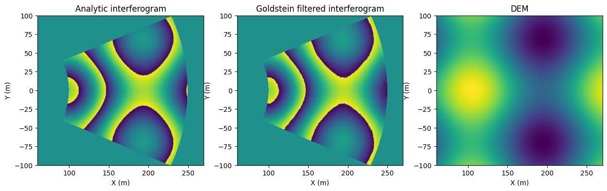
Cartesian projection

Above images are in pseudo-polar coordinates. We can project them to Cartesian plane to compare with DEM. Interferograms are still wrapped, but their shape can be compared to DEM.

analytic_cart = torchbp.ops.polar_to_cart(analytic_wrapped, origin0, grid_polar, grid_proj, fc=0)[0]
gold_cart = torchbp.ops.polar_to_cart(torch.angle(inf_gold), origin0, grid_polar, grid_proj, fc=0)[0]

fig, axes = plt.subplots(1, 3, figsize=(15, 4))
axes[0].imshow(analytic_cart.T.cpu().numpy(), origin="lower", extent=extent_proj, aspect="auto", vmin=-np.pi, vmax=np.pi)
axes[0].set_xlabel("X (m)")
axes[0].set_ylabel("Y (m)")
axes[0].set_title("Analytic interferogram")

axes[1].imshow(gold_cart.T.cpu().numpy(), origin="lower", extent=extent_proj, aspect="auto", vmin=-np.pi, vmax=np.pi)
axes[1].set_xlabel("X (m)")
axes[1].set_ylabel("Y (m)")
axes[1].set_title("Goldstein filtered interferogram")

axes[2].imshow(dem.cpu().numpy().T, origin="lower", extent=extent_proj, aspect="auto")
axes[2].set_xlabel("X (m)")
axes[2].set_ylabel("Y (m)")
axes[2].set_title("DEM");