Antenna-pattern-aware image formation

A radar with a narrow azimuth beam (a scanning / stripmap-style acquisition) only illuminates each ground point for the short part of the aperture when the beam sweeps past it. During the rest of the aperture that point receives almost no signal, just noise.

If the image is backprojected with every pulse weighted equally, those many low-gain pulses add noise into each pixel. With antenna pattern and pointing informtion (g, g_extent, att) it’s possible to weight each pulse according to the gain toward that pixel.

Both torchbp.ops.backprojection_polar_2d and torchbp.ops.ffbp accept the antenna pattern. This example uses ffbp and compares image formation with and without the antenna pattern on a noisy scanning acquisition.

import math
import torch
import numpy as np
import matplotlib.pyplot as plt
from numpy import hamming

import torchbp

device = "cuda" if torch.cuda.is_available() else "cpu"
print("Device:", device)
torch.manual_seed(0);

Device: cpu

Acquisition geometry

A small FMCW radar flies along \(y\) at 30 m altitude, looking toward \(+x\). The azimuth is sampled at the Nyquist rate (element spacing \(\lambda/4\)). Few point targets are spread across the swath so we can watch the beam sweep over each in turn.

fc = 6e9            # RF center frequency (Hz)
bw = 200e6          # Sweep bandwidth (Hz)
tsweep = 100e-6     # Sweep length (s)
fs = 4e6            # Sampling frequency (Hz)
nsamples = int(fs * tsweep)
nsweeps = 512       # Pulses in the aperture
oversample = 2      # Range FFT oversampling
wl = 3e8 / fc
element_spacing = 0.25 * wl   # Nyquist azimuth sampling
altitude = 30.0

# Point targets across the swath, all at 120 m ground range.
r_mid = 120.0
target_y = torch.tensor([-45.0, 0.0, 45.0], device=device)
target_pos = torch.stack([torch.full_like(target_y, r_mid), target_y,
                          torch.zeros_like(target_y)], dim=1)
target_rcs = torch.ones((target_y.numel(), 1), dtype=torch.float32, device=device)

# Straight track along y.
pos = torch.zeros((nsweeps, 3), dtype=torch.float32, device=device)
pos[:, 1] = torch.linspace(-nsweeps / 2, nsweeps / 2, nsweeps, device=device) * element_spacing
pos[:, 2] = altitude

grid = {"r": (95.0, 145.0), "theta": (-0.55, 0.55), "nr": 256, "ntheta": 512}

Antenna pattern and beam steering

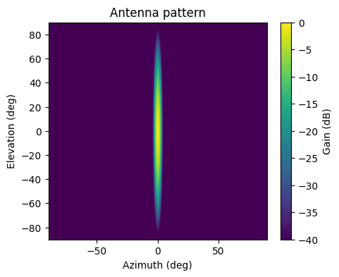
A tight pencil beam: narrow in azimuth, broad in elevation. The pattern g is the square root of the two-way gain on an elevation x azimuth grid, with extent g_extent = [el0, az0, el1, az1] in radians. During the pass the antenna yaw is swept linearly across ±25°, scanning the beam over the whole swath. A fixed roll points the elevation beam down at mid-swath.

naz, nel = 256, 64
az = np.linspace(-np.pi / 2, np.pi / 2, naz)
el = np.linspace(-np.pi / 2, np.pi / 2, nel)
az_bw = np.deg2rad(2)     # azimuth beamwidth
el_bw = np.deg2rad(40)    # elevation beamwidth
gain = np.exp(-(el[:, None] / el_bw) ** 2) * np.exp(-(az[None, :] / az_bw) ** 2)
g = torch.tensor(gain, dtype=torch.float32, device=device)
g_extent = [el[0], az[0], el[-1], az[-1]]

roll = -np.arctan2(altitude, r_mid) # point elevation beam to mid-swath
att = torch.zeros_like(pos)
att[:, 0] = roll
att[:, 2] = torch.linspace(-np.deg2rad(25), np.deg2rad(25), nsweeps, device=device)  # yaw sweep

plt.figure(figsize=(5, 4))
plt.imshow(20 * np.log10(gain + 1e-6), origin="lower", aspect="auto",
           extent=[np.rad2deg(az[0]), np.rad2deg(az[-1]), np.rad2deg(el[0]), np.rad2deg(el[-1])],
           vmin=-40, vmax=0)
plt.colorbar(label="Gain (dB)")
plt.xlabel("Azimuth (deg)"); plt.ylabel("Elevation (deg)"); plt.title("Antenna pattern");

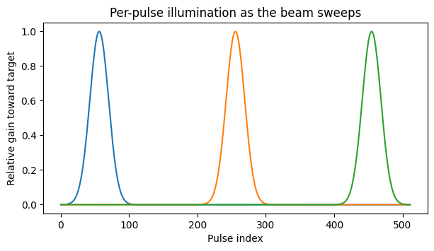
Each target is illuminated only briefly

As the beam yaw sweeps, the gain toward a fixed target rises and falls. Outside it the target contributes essentially no signal, so those pulses carry only noise into the backprojection sum.

pos_y = pos[:, 1].cpu().numpy()
yaw = att[:, 2].cpu().numpy()
plt.figure(figsize=(7, 3.5))
for ty in target_y.cpu().numpy():
    az_to_target = np.arctan2(ty - pos_y, r_mid) - yaw
    gk = np.exp(-(az_to_target / az_bw) ** 2)
    plt.plot(np.arange(nsweeps), gk, label=f"target y={ty:+.0f} m")
plt.xlabel("Pulse index"); plt.ylabel("Relative gain toward target")
plt.title("Per-pulse illumination as the beam sweeps");

Simulate the data and add noise

The beat signals are generated with the antenna pattern and attitude, range-compressed (windowed, oversampled IFFT, spectrum centered with data_fmod), then thermal noise is added in the range-compressed domain.

raw = torchbp.util.generate_fmcw_data(target_pos, target_rcs, pos, fc, bw, tsweep, fs,
                                      g=g, g_extent=g_extent, att=att)
w = torch.tensor(hamming(raw.shape[-1])[None, :], dtype=torch.float32, device=device)
clean = torch.fft.ifft(raw * w, dim=-1, n=nsamples * oversample)
data_fmod = -math.pi * (1 - (oversample - 1) / oversample)
clean = clean * torch.exp(1j * data_fmod * torch.arange(clean.shape[-1], device=device))[None, :]
r_res = 3e8 / (2 * bw * oversample)

# Add noise
sigma = clean.abs().pow(2).mean().sqrt()
torch.manual_seed(7)
noise = 30 * sigma / math.sqrt(2) * (torch.randn_like(clean.real) + 1j * torch.randn_like(clean.real))

Form the image, with and without the antenna pattern

Backprojection is linear, so ffbp(clean + noise) = ffbp(clean) + ffbp(noise). We form the signal-only and noise-only images for each method. Their sum is the noisy image to display, and they also give a clean per-target SNR. The uniform is given no antenna information and the antenna-aware gets att, g, g_extent.

def form(data, weighted):
    kw = dict(data_fmod=data_fmod, dealias=True)
    if weighted:
        kw.update(att=att, g=g, g_extent=g_extent)
    return torchbp.ops.ffbp(data, grid, fc, r_res, pos, stages=3, divisions=2, **kw).squeeze()

S_uni, N_uni = form(clean, False), form(noise, False)   # uniform: signal, noise
S_ant, N_ant = form(clean, True),  form(noise, True)    # antenna-aware: signal, noise
img_uni = S_uni + N_uni
img_ant = S_ant + N_ant

extent = [*grid["r"], *grid["theta"]]
fig, axes = plt.subplots(1, 2, figsize=(13, 4.5))
vmax = 20 * torch.log10(img_ant.abs() + 1e-12).max().item()
for ax, im, title in zip(axes, [img_uni, img_ant],
                         ["Uniform (no antenna pattern)", "Antenna-aware"]):
    db = 20 * torch.log10(im.abs() + 1e-12).cpu().numpy()
    h = ax.imshow(db.T, origin="lower", vmin=vmax - 30, vmax=vmax, extent=extent, aspect="auto")
    ax.set_title(title); ax.set_xlabel("Range (m)")
    plt.colorbar(h, ax=ax, label="dB")
axes[0].set_ylabel("Angle (sin)")
plt.tight_layout(); plt.show()

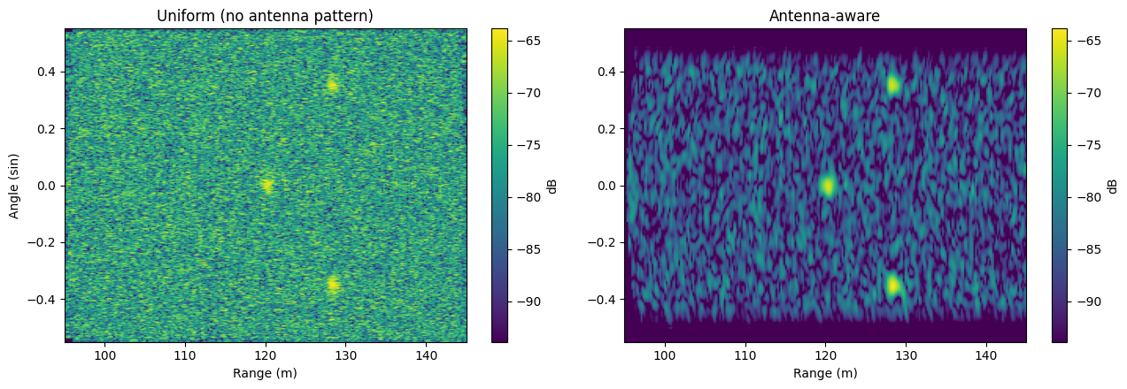
The targets stand out more cleanly against the noise in the antenna-aware image.

Per-target SNR

Using the separate signal and noise images, SNR at each target is the signal peak over the local RMS of the noise image at that pixel.

def find_peaks(I, n):
    m = I.abs().cpu().numpy().copy(); pts = []
    for _ in range(n):
        ri, ci = np.unravel_index(m.argmax(), m.shape); pts.append((ri, ci))
        m[max(0, ri-12):ri+12, max(0, ci-12):ci+12] = 0
    return sorted(pts, key=lambda p: p[1])

print("target  |  uniform  | antenna-aware |  gain")
for ri, ci in find_peaks(S_uni, target_y.numel()):
    nu = N_uni[ri-8:ri+8, ci-8:ci+8].abs().std().item()
    na = N_ant[ri-8:ri+8, ci-8:ci+8].abs().std().item()
    snr_u = 20 * math.log10(S_uni[ri, ci].abs().item() / nu)
    snr_a = 20 * math.log10(S_ant[ri, ci].abs().item() / na)
    print(f"  c{ci:>4} | {snr_u:6.1f} dB | {snr_a:10.1f} dB | {snr_a - snr_u:+5.1f} dB")

target  |  uniform  | antenna-aware |  gain
  c  93 |   15.8 dB |       23.4 dB |  +7.6 dB
  c 256 |   16.5 dB |       25.2 dB |  +8.7 dB
  c 419 |   15.2 dB |       25.8 dB | +10.6 dB

Every target gains several dB. The improvement is the matched-filter gain \(N\,\Sigma g_k^2 / (\Sigma g_k)^2\). The antenna-aware image formation effectively integrates only the pulses that actually saw the target, instead of diluting the signal with noise-only pulses.