Fast factorized backprojection (FFBP)

Direct backprojection forms a SAR image by summing, for every output pixel, the contribution of every pulse in the aperture. It asymptotic scaling is therefore \(\mathcal{O}(NRA)\), where \(N\) is the number of pulses, \(R\) is the number of range pixels, and \(A\) is the number of azimuth pixels. The number of azimuth pixels also scales linearly with number of pulses for linear track, so we can say that the algoritm is \(\mathcal{O}(N^2)\).

Fast factorized backprojection (FFBP) reduces this cost. The idea is:

1. Split the aperture into short subapertures. A short subaperture has a small angular (Doppler) bandwidth, so its image can be formed on a coarse polar grid

2. Coherently merge pairs of subaperture images onto a finer grid repeating in a binary tree. Each merge doubles the azimuth resolution (and doubles the image azimuth size)

At the limit of many recursion stages, the asymptotic cost is \(\mathcal{O}(N \log N)\).

The library exposes this as a single call, torchbp.ops.ffbp. In this notebook the algorithm is built by hand from the low-level ops to demonstrate how it works. backprojection_polar_2d is used to form the lowest-level subapertures and the ffbp_merge2 op is use to recursively merge the images.

import math
import torch
import numpy as np
import matplotlib.pyplot as plt
from numpy import hamming

import torchbp
from torchbp.util import center_pos
from torchbp.ops import backprojection_polar_2d, ffbp_merge2

device = "cuda" if torch.cuda.is_available() else "cpu"
print("Device:", device)

Device: cpu

Scene and radar parameters

A single point target, imaged on a heavily oversampled polar grid zoomed around the target so the point-spread function (PSF) is smooth and easy to inspect. The aperture is split into a power-of-two number of subapertures, so we use nsweeps = 512. ffbp can also handle non power-of-two nsweeps efficiently, but this choice simplifies the example.

fc = 6e9          # RF center frequency (Hz)
bw = 200e6        # RF bandwidth (Hz), positive for rising sweep
tsweep = 100e-6   # Sweep length (s)
fs = 2e6          # Sampling frequency (Hz)
nsweeps = 512     # Number of pulses in the aperture
oversample = 2    # Range FFT oversampling (reduces interpolation error)
nsamples = int(fs * tsweep)

# Heavily oversampled polar grid, zoomed on the target. theta is sin(angle).
nr, ntheta = 256, 512
grid = {"r": (96.0, 104.0), "theta": (-0.06, 0.06), "nr": nr, "ntheta": ntheta}

# Single point target at 100 m, broadside.
target_pos = torch.tensor([[100.0, 0.0, 0.0]], dtype=torch.float32, device=device)
target_rcs = torch.ones((1, 1), dtype=torch.float32, device=device)

# Straight platform track along y at 50 m height. Element spacing = lambda/4.
pos = torch.zeros((nsweeps, 3), dtype=torch.float32, device=device)
pos[:, 1] = torch.linspace(-nsweeps / 2, nsweeps / 2, nsweeps, device=device) * 0.25 * 3e8 / fc
pos[:, 2] = 50.0

Simulate and range-compress the data

Identical to the backprojection example. Generate raw data, apply a range window, and FFT to range-compress. data_fmod shifts the data spectrum to DC and alias_fmod centers the image spectrum. Both reduce interpolation error and must be passed consistently to backprojection and the FFBP merge.

raw = torchbp.util.generate_fmcw_data(target_pos, target_rcs, pos, fc, bw, tsweep, fs)
w = torch.tensor(hamming(raw.shape[-1])[None, :], dtype=torch.float32, device=device)
data = torch.fft.ifft(raw * w, dim=-1, n=nsamples * oversample)

data_fmod = -math.pi * (1 - (oversample - 1) / oversample)
data = data * torch.exp(1j * data_fmod * torch.arange(data.shape[-1], device=device))[None, :]

r_res = 3e8 / (2 * abs(bw) * oversample)           # range bin size in the data
dr = (grid["r"][1] - grid["r"][0]) / grid["nr"]    # range bin size in the image
im_margin = oversample * r_res / dr - 1
alias_fmod = -math.pi * (1 - im_margin / (1 + im_margin))
print(f"r_res={r_res:.3f} m, image dr={dr:.3f} m, data_fmod={data_fmod:.3f}, alias_fmod={alias_fmod:.3f}")

r_res=0.375 m, image dr=0.031 m, data_fmod=-1.571, alias_fmod=-0.131

A small helper to display a polar image in dB.

extent = [*grid["r"], *grid["theta"]]

def show_polar(img, title, ax=None, dyn=30, ref_max=None):
    img = img.detach().cpu()
    db = 20 * torch.log10(torch.abs(img) + 1e-12)
    m = db.max() if ref_max is None else ref_max
    if ax is None:
        _, ax = plt.subplots()
    im = ax.imshow(db.numpy().T, origin="lower", vmin=m - dyn, vmax=m,
                   extent=extent, aspect="auto")
    ax.set_title(title)
    ax.set_xlabel("Range (m)")
    ax.set_ylabel("Angle (sin)")
    return m

def relerr(a, b):
    return (torch.linalg.norm(a - b) / torch.linalg.norm(a)).item()

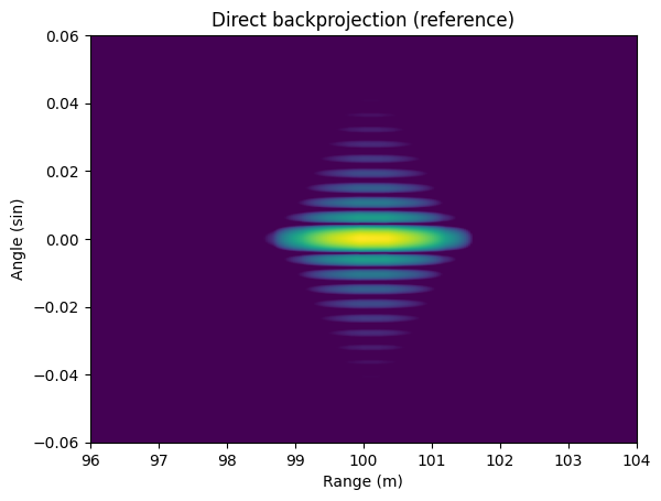
Reference: Direct backprojection

img_bp = backprojection_polar_2d(
    data, grid, fc, r_res, pos, dealias=True, data_fmod=data_fmod, alias_fmod=alias_fmod
).squeeze()

m = show_polar(img_bp, "Direct backprojection (reference)")
plt.show()

Step 1: Backproject the subapertures (coarse azimuth)

Split the aperture in two halves. Each half is backprojected on its own local polar frame, centered on that half’s mean antenna phase center (APC) with center_pos. Because each half spans only half the aperture, its azimuth bandwidth is halved, so half as many azimuth samples suffice. Since backprojection scales quadratically with number of sweeps, generating two coarser images from both halves of the data is 2x faster than generating the full resolution image. We keep a small internal oversampling factor to limit interpolation errors at the edges during the later merge.

OSR = 1.4  # internal oversampling of subaperture grids (limits interpolation error)

def backproject_subaperture(sl, ntheta_sub):
    """Backproject the pulses in slice `sl` onto a local coarse-azimuth polar grid."""
    p = pos[sl]
    p_local, origin = center_pos(p)
    g = {"r": grid["r"], "theta": grid["theta"],
         "nr": int(OSR * nr), "ntheta": int(OSR * ntheta_sub)}
    img = backprojection_polar_2d(
        data[sl], g, fc, r_res, p_local,
        dealias=True, data_fmod=data_fmod, alias_fmod=alias_fmod,
    ).squeeze()
    return {"img": img, "grid": g, "origin": origin[0], "z": p[:, 2].mean()}

half = nsweeps // 2
subA = backproject_subaperture(slice(0, half), ntheta // 2)
subB = backproject_subaperture(slice(half, nsweeps), ntheta // 2)

print("subaperture image shape:", tuple(subA["img"].shape), "(full grid is", (nr, ntheta), ")")
fig, axs = plt.subplots(1, 2, figsize=(11, 4))
show_polar(subA["img"], "Subaperture A (first half)", ax=axs[0])
show_polar(subB["img"], "Subaperture B (second half)", ax=axs[1])
plt.tight_layout(); plt.show()

subaperture image shape: (358, 358) (full grid is (256, 512) )

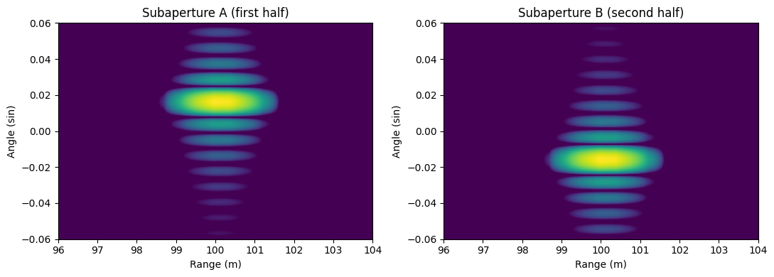
Each subaperture image is correctly focused but resolution is not as good as in the reference, since only half of the data is used. The main lobe is about twice as wide as in the reference. The two images also sit at different coordinate frames, each referenced to its own APC.

Step 2: Merge

ffbp_merge2 interpolates the two subaperture images onto a common, finer output grid referenced to the combined APC, and sums them coherently. To do that it needs, for each input, the vector from its origin to the new origin (dorigin, with the height component handled separately) and the carrier frequency fc to keep the phases consistent. Combining the two halves restores the full azimuth bandwidth, hence full resolution.

ffbp_merge2 is essentially the same operation as polar_interp, but merges the two interpolations in one kernel for faster execution. It uses Knab pulse interpolation that is almost optimal finite interpolation kernel, when the oversampling rate is known. (J. Knab, “The sampling window,” in IEEE Transactions on Information Theory, vol. 29, no. 1, pp. 157-159, January 1983.)

def merge(a, b, grid_new):
    new_origin = 0.5 * (a["origin"] + b["origin"])
    new_z = 0.5 * (a["z"] + b["z"])
    da = (new_origin - a["origin"]).clone(); da[2] = -(new_z - a["z"])
    db = (new_origin - b["origin"]).clone(); db[2] = -(new_z - b["z"])
    img = ffbp_merge2(
        a["img"], b["img"], da, db, [a["grid"], b["grid"]], fc, grid_new,
        z0=float(new_z), method=("knab", 6, 1.5),
        alias=False, alias_fmod=alias_fmod, output_alias=True,
    )
    return {"img": img.squeeze(), "grid": grid_new, "origin": new_origin, "z": new_z}

img_ffbp2 = merge(subA, subB, grid)["img"]

fig, axs = plt.subplots(1, 2, figsize=(11, 4))
show_polar(img_bp, "Direct backprojection", ax=axs[0], ref_max=m)
show_polar(img_ffbp2, "FFBP, 2 subapertures (manual)", ax=axs[1], ref_max=m)
plt.tight_layout(); plt.show()

print(f"relative error vs direct BP: {relerr(img_bp, img_ffbp2):.4f}")

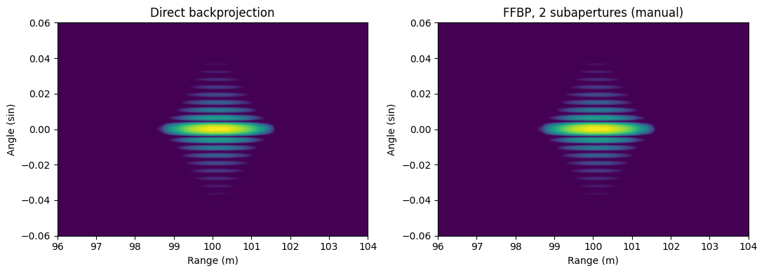
relative error vs direct BP: 0.0543

The merged image matches the reference. Azimuth cut overlays perfectly. The largest error is near the edges caused by edge effects from interpolation.

pk = np.unravel_index(torch.abs(img_bp).cpu().argmax(), img_bp.shape)
theta_axis = np.linspace(grid["theta"][0], grid["theta"][1], ntheta)
cut_bp = 20 * torch.log10(torch.abs(img_bp[pk[0]]).cpu() + 1e-12)
cut_ff = 20 * torch.log10(torch.abs(img_ffbp2[pk[0]]).cpu() + 1e-12)

fig, axs = plt.subplots(1, 2, figsize=(12, 4))
axs[0].plot(theta_axis, cut_bp - cut_bp.max(), label="direct BP")
axs[0].plot(theta_axis, cut_ff - cut_bp.max(), "--", label="FFBP (manual)")
axs[0].set_xlim(-0.02, 0.02); axs[0].set_ylim(-40, 1)
axs[0].set_xlabel("Angle (sin)"); axs[0].set_ylabel("dB")
axs[0].set_title("Azimuth cut through peak"); axs[0].legend()
show_polar(img_bp - img_ffbp2, "Difference (FFBP - direct)", ax=axs[1], ref_max=m, dyn=50)
plt.tight_layout(); plt.show()

/tmp/ipykernel_3491/859417228.py:1: DeprecationWarning: __array__ implementation doesn't accept a copy keyword, so passing copy=False failed. __array__ must implement 'dtype' and 'copy' keyword arguments. To learn more, see the migration guide https://numpy.org/devdocs/numpy_2_0_migration_guide.html#adapting-to-changes-in-the-copy-keyword
  pk = np.unravel_index(torch.abs(img_bp).cpu().argmax(), img_bp.shape)

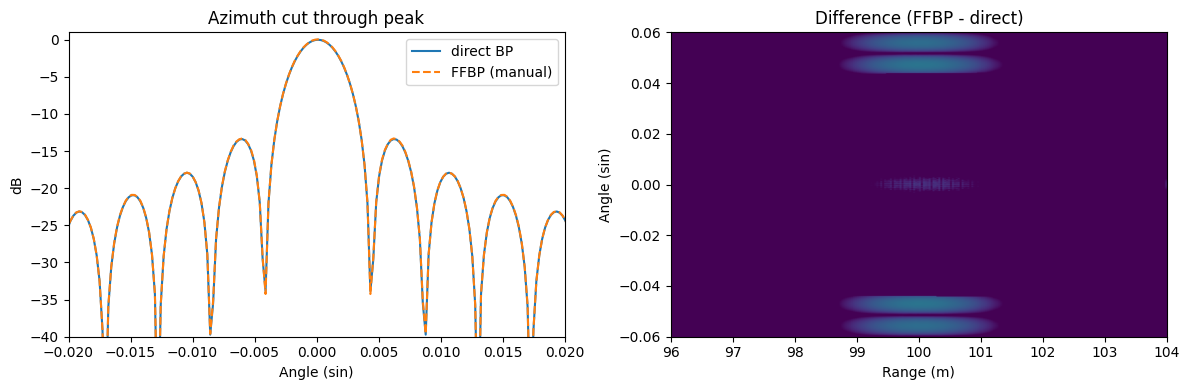
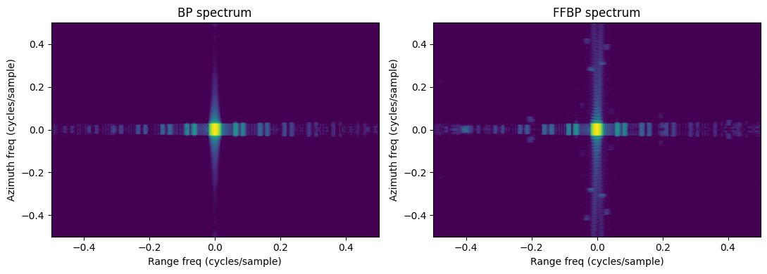
Spectrum of both images. FFBP interpolation error spreads the spectrum a little bit in azimuth. Range aliasing comes from linear interpolation used in backprojection.

spec_bp_db = 20*np.log10(np.abs(np.fft.fftshift(np.fft.fft2(img_bp)))).T
ms = np.max(spec_bp_db)

fig, axes = plt.subplots(1, 2, figsize=(11, 4))
axes[0].imshow(spec_bp_db, origin="lower", aspect="auto", vmax=ms, vmin=ms - 80, extent=[-0.5, 0.5, -0.5, 0.5])
axes[0].set_xlabel("Range freq (cycles/sample)")
axes[0].set_ylabel("Azimuth freq (cycles/sample)")
axes[0].set_title("BP spectrum");

spec_ff_db = 20*np.log10(np.abs(np.fft.fftshift(np.fft.fft2(img_ffbp2)))).T

axes[1].imshow(spec_ff_db, origin="lower", aspect="auto", vmax=ms, vmin=ms - 80, extent=[-0.5, 0.5, -0.5, 0.5])
axes[1].set_xlabel("Range freq (cycles/sample)")
axes[1].set_ylabel("Azimuth freq (cycles/sample)")
axes[1].set_title("FFBP spectrum")
plt.tight_layout();

Recursion

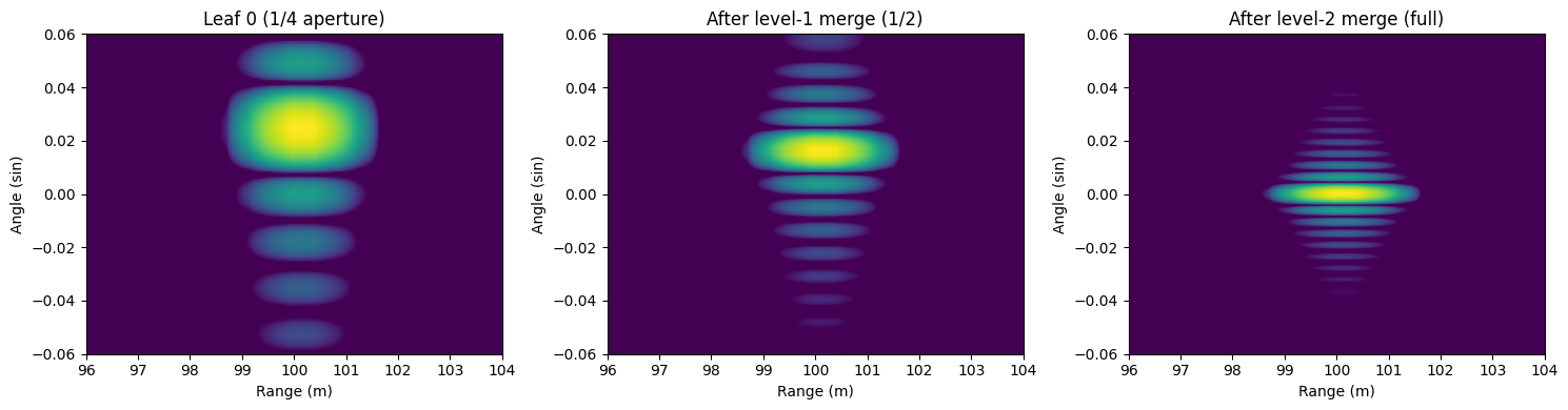
One merge halves the work of the azimuth dimension, the real speedup comes from recursing. With four subapertures we backproject four coarse images and merge them in a two-level binary tree: merge A+B and C+D to half-resolution intermediates, then merge those two to the full image. In general \(N_\text{sub}\) subapertures need \(\log_2 N_\text{sub}\) merge stages.

NSUB = 4
n = nsweeps // NSUB
leaves = [backproject_subaperture(slice(i * n, (i + 1) * n), ntheta // NSUB)
          for i in range(NSUB)]

# Level 1: merge pairs onto half-resolution intermediate grids.
grid_mid = {"r": grid["r"], "theta": grid["theta"],
            "nr": int(OSR * nr), "ntheta": int(OSR * (ntheta // 2))}
mid0 = merge(leaves[0], leaves[1], grid_mid)
mid1 = merge(leaves[2], leaves[3], grid_mid)

# Level 2: merge the intermediates onto the full output grid.
img_ffbp4 = merge(mid0, mid1, grid)["img"]

fig, axs = plt.subplots(1, 3, figsize=(15, 4))
show_polar(leaves[0]["img"], "Leaf 0 (1/4 aperture)", ax=axs[0])
show_polar(mid0["img"], "After level-1 merge (1/2)", ax=axs[1])
show_polar(img_ffbp4, "After level-2 merge (full)", ax=axs[2], ref_max=m)
plt.tight_layout(); plt.show()

print(f"4-subaperture FFBP, relative error vs direct BP: {relerr(img_bp, img_ffbp4):.4f}")

4-subaperture FFBP, relative error vs direct BP: 0.0765

The azimuth resolution sharpens at each merge. The four-leaf result is still visually focused, but its residual is larger than the two-leaf case, because every merge interpolates and those errors accumulate with tree depth. This is the central trade-off of FFBP.

The point target is at different azimuth angles in different images, since the image origin is at the center of the data that is processed.

Library op torchbp.ops.ffbp

Everything above is what torchbp.ops.ffbp does internally. stages is the number of recursion levels. It should match the hand-built results.

img_lib1 = torchbp.ops.ffbp(data, grid, fc, r_res, pos, stages=1, divisions=2,
                            data_fmod=data_fmod, alias_fmod=alias_fmod, dealias=True).squeeze()
img_lib2 = torchbp.ops.ffbp(data, grid, fc, r_res, pos, stages=2, divisions=2,
                            data_fmod=data_fmod, alias_fmod=alias_fmod, dealias=True).squeeze()

print(f"stages=1 vs manual 2-subaperture: {relerr(img_ffbp2, img_lib1):.4f}")
print(f"stages=2 vs manual 4-subaperture: {relerr(img_ffbp4, img_lib2):.4f}")
print(f"stages=1 vs direct BP:            {relerr(img_bp, img_lib1):.4f}")
print(f"stages=2 vs direct BP:            {relerr(img_bp, img_lib2):.4f}")

stages=1 vs manual 2-subaperture: 0.0039
stages=2 vs manual 4-subaperture: 0.0000
stages=1 vs direct BP:            0.0543
stages=2 vs direct BP:            0.0765

Benefit and downside

Benefit: FFBP is asymptotically faster and the difference can be huge for large image (10 to 100x faster for realistic size image).

Downside: interpolation error. Each merge resamples the images with a finite interpolation kernel and the error accumulates with the number of stages. The error can be reduced with higher-order interpolation kernel (interp_method=("knab", order, oversample)) and larger internal oversampling (oversample_r, oversample_theta), but both of these increase the amount of work. In practice, number of stages, interpolation kernel size, and oversampling factor needs to be chosen based on the maximum allowed error in the final result.