Choosing fc for backprojection

fc in backprojection is the carrier of the per-pixel phase compensation $e^{+j 4\pi f_c R / c}$ applied to the range-compressed data. It must match the phase-reference convention of the data, and that convention is set by the waveform and how the range profile is read out:

Interpolating readout (= backprojection): reference = first ADC sample, so fc = flow for a rising sweep, fc = fhigh for a falling sweep.
Interpolating readout + mid-sweep factor $e^{-j\pi f T}$: reference = mid sweep, so fc = fcenter, both sweep directions.
Rising sweep, ADC samples time-reversed: reference = last ADC sample, so fc = flow + K(N-1)/fs ≈ fhigh.
Rising sweep, delayed ADC start: reference = first ADC sample, so fc = the frequency at that first sample.
FFT + fixed range bin (classic range–Doppler analysis): reference = window centre (via leakage), so fc = fcenter.
Matched-filter pulse compression, DC-centred baseband: reference = demodulation frequency (LO), so fc = fcenter.

flow is the lowest frequency (start frequency for rising sweep) and fhigh is the highest frequency. For falling sweep the start frequency is fhigh.

“Phase reference at the first ADC sample” is a property of the readout, not of the signal: the FFT correlates the whole windowed sweep against $e^{-j2\pi f t}$, whose zero-phase instant is the first sample, so the measured phase is a fit to the entire sweep, quoted at that instant. fc = flow is not a sampling of the hardware frequency at one instant: sweep non-linearity matters through its window-weighted effect over the whole sweep and its value at the reference instant specifically carries no special weight. Only a deviation with a nonzero window-weighted mean shifts the effective reference.

This example demonstrates:

RF-sample-level simulation: the dechirped IF signal is $e^{\,j 2\pi (f_{low}\tau + K\tau t - K\tau^2/2)}$ with $t = 0$ at the first ADC sample. A plain FFT therefore leaves the data referenced to the sweep start, and backprojection must use fc = flow for a rising sweep.
fc is phase bookkeeping: even a hypothetical DC-start sweep (flow = 0, so fc = 0 and the phase compensation is identically 1) focuses perfectly. Azimuth resolution is set by the physical spectrum of the signal, not by the fc parameter.
Mid-sweep re-referencing: multiplying the conjugated range spectrum by $e^{-j\pi f T}$ (over the signed beat-frequency axis $f$, sweep length $T$) moves the reference to mid sweep, making fc = fcenter exact and rising/falling sweeps symmetric, so identical processing handles both sweep directions.
Time reversal: reversing the ADC samples moves the phase reference to the frequency at the last sample in the original order. fc must be changed to correctly focus the image for start-referenced signal.
Why fixed-bin analyses mislead: reading the phase history from one fixed FFT bin while the target migrates through range bins is fcenter-referenced through window leakage. This is how classical range-Doppler processing works. That is a property of that readout, not of backprojection, which interpolates at the beat frequency.
Pulse compression radar: correlation range compression time origin moves the range origin, not the phase reference. fc equals the demodulation frequency, fcenter for the usual DC-centred baseband convention, regardless of window placement or sample order.

Dechirp signal model

Rising-sweep TX phase with chirp rate $K = B/T$:

\[\varphi_{tx}(t) = 2\pi\!\left(f_{low}\,t + \tfrac{1}{2}K t^2\right)\]

The mixer forms IF $=$ TX $\cdot$ conj(RX) with RX $=$ TX$(t-\tau)$, $\tau = 2R/c$:

\[\varphi_{IF}(t) = \varphi_{tx}(t) - \varphi_{tx}(t-\tau) = 2\pi\!\left(f_{low}\,\tau + K\tau\,t - \tfrac{1}{2}K\tau^2\right), \qquad t = 0 \text{ at the first ADC sample.}\]

Re-parameterizing the same signal about mid sweep, $t' = t - T/2$, gives $2\pi(f_c\tau + K\tau t' - \tfrac12 K\tau^2)$ with $f_c = f_{low} + B/2$, identical signal but different fc. The choice of where $t=0$ affects the required fc value and this depends on the processing method.

Range compression with the Fourier transform basis $e^{-j2\pi f t}$ ($t=0$ at the first sample), evaluated at the beat frequency $f_b = K\tau$, which is what backprojection’s interpolation does, leaves

\[\angle X(f_b) = 2\pi f_{low}\tau - \pi K \tau^2 .\]

In the conjugated-spectrum convention (assuming rising sweep) the target phase is $-4\pi f_{low} R/c + \pi K\tau^2$, so the backprojection compensation $e^{+j4\pi f_c R/c}$ cancels it only if fc = $f_{low}$. The last term ($ -\pi `K :nbsphinx-math:tau`^2$) is the residual video phase (RVP): small, common to every fc choice. It can be compensated separately if necessary.

Mid-sweep factor: on the conjugated spectrum the target sits at $f = K\tau$, so multiplying by $e^{-j\pi f T}$ contributes $e^{-j\pi K\tau T} = e^{-j\pi B\tau}$, moving the reference phase to $-4\pi(f_{low}+B/2)R/c$: exactly $f_c = f_{center}$. A falling sweep puts the target at $f = -K\tau$ and the same factor yields $-4\pi(f_{stop}-B/2)R/c$ — again $f_{center}$. One factor, both sweep directions.

[1]:

import numpy as np
from scipy import signal
import torch
import torchbp
import matplotlib.pyplot as plt
from numpy import hamming, hanning

c0 = 3e8

RF-sample-level FMCW simulation

TX chirp sampled at 8 GHz, delayed RX, calculate mixer product, zero-phase low-pass filter (no delay to avoid modifying phase), analytic signal, decimation to the 50 MHz ADC rate. No complex-exponential shortcuts used.

A realistic sweep (1.0–1.5 GHz) is used here because a real mixer cannot dechirp a DC-start sweep: near $t \approx \tau$ the sum and difference products overlap at DC and no filter separates them. That is also why the DC-start sweep used later is hypothetical, there it is generated directly from the analytic IF model that this part validates.

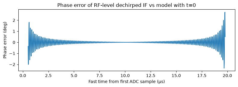
Lowpass filtering causes slight error at the edges because of edge-effects, but the match is good against the ideal IF signal.

[2]:

flow = 1.0e9 # sweep 1.0 -> 1.5 GHz
bw1 = 0.5e9
tsweep1 = 20e-6
K1 = bw1 / tsweep1
fc1 = flow + bw1 / 2

fs_rf = 8e9 # RF simulation rate
n_rf = int(round(tsweep1 * fs_rf))
t_rf = np.arange(n_rf) / fs_rf
dec = 160
fs_adc = fs_rf / dec # 50 MHz ADC
n_adc = n_rf // dec
t_adc = np.arange(n_adc) / fs_adc
phi0 = 0.1234 # Arbitrary TX phase offset

def phi_tx(t):
    return 2 * np.pi * (flow * t + 0.5 * K1 * t**2) + phi0

def rf_dechirp(tau):
    '''TX, delayed RX, mixer, LPF, Hilbert, decimate.'''
    tx = np.cos(phi_tx(t_rf))
    rx = np.where(t_rf >= tau, np.cos(phi_tx(t_rf - tau)), 0.0)
    b, a = signal.butter(6, 20e6 / (fs_rf / 2))
    beat = signal.filtfilt(b, a, tx * rx) # zero-phase LPF
    return signal.hilbert(beat)[::dec]

R_test = 45.0
tau_test = 2 * R_test / c0
sig = rf_dechirp(tau_test)

# analytic IF model, t = 0 at the first ADC sample
phi_model = 2 * np.pi * (flow * tau_test + K1 * tau_test * t_adc
                         - 0.5 * K1 * tau_test**2)
valid = (t_adc > tau_test + 200e-9) & (t_adc < tsweep1 - 200e-9)
perr = np.angle(sig * np.exp(-1j * phi_model))
print(f"R = {R_test} m, tau = {tau_test*1e9:.1f} ns, "
      f"beat = {K1*tau_test/1e6:.2f} MHz")
print(f"IF phase error vs first-sample model: "
      f"RMS {np.sqrt(np.mean(perr[valid]**2))*1e3:.2f} mrad, "
      f"max {np.max(np.abs(perr[valid]))*1e3:.2f} mrad")

# sanity check: the mid-sweep parameterization is the SAME signal
phi_mid = 2 * np.pi * (fc1 * tau_test + K1 * tau_test * (t_adc - tsweep1 / 2)
                       - 0.5 * K1 * tau_test**2)

print(f"first-sample vs mid-sweep parameterization: max difference "
      f"{np.max(np.abs(phi_model - phi_mid)):.2e} rad")
print("   (identical signal to float rounding)")

plt.figure(figsize=(8, 3))
plt.plot(t_adc[valid] * 1e6, perr[valid] * 180/np.pi)
plt.xlabel("Fast time from first ADC sample (µs)")
plt.ylabel("Phase error (deg)")
plt.title("Phase error of RF-level dechirped IF vs model with t=0")
plt.tight_layout()

R = 45.0 m, tau = 300.0 ns, beat = 7.50 MHz
IF phase error vs first-sample model: RMS 5.97 mrad, max 47.58 mrad
first-sample vs mid-sweep parameterization: max difference 4.55e-13 rad
   (identical signal to float rounding)

Which reference does the interpolating readout leave?

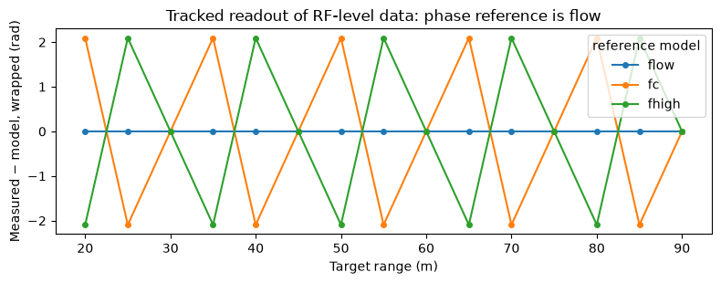
Repeat the RF-level simulation at different target distances and read the (windowed, conjugated) DTFT out at the beat frequency, exactly what backprojection’s interpolation does. The measured phase is compared against the candidate models $-2\pi f_{ref}\tau + \pi K\tau^2$. The candidates are far apart ($f_c$ vs $f_{low}$ differ by $2\pi (B/2)\tau \approx$ hundreds of radians here), so the verdict is unambiguous: flow is the correct choice.

[3]:

Rs = np.linspace(20, 90, 15)
taus = 2 * Rs / c0
win = hanning(n_adc)
n = np.arange(n_adc)
meas = np.empty(len(Rs))
for i, tau in enumerate(taus):
    s = rf_dechirp(tau)
    fb = K1 * tau
    X = (win * s * np.exp(-2j * np.pi * fb * n / fs_adc)).sum().conj()
    meas[i] = np.angle(X)

plt.figure(figsize=(8, 3.2))
for name, f_ref in {"flow": flow, "fc": fc1, "fhigh": flow + bw1}.items():
    model = -2 * np.pi * f_ref * taus + np.pi * K1 * taus**2
    d = np.angle(np.exp(1j * (meas - model)))
    print(f"readout phase vs {name:6s} model: wrapped-difference "
          f"RMS {np.sqrt(np.mean(d**2)):7.4f} rad")
    plt.plot(Rs, d, "o-", ms=4, label=name)
plt.xlabel("Target range (m)")
plt.ylabel("Measured − model, wrapped (rad)")
plt.title("Tracked readout of RF-level data: phase reference is flow")
plt.legend(title="reference model")
plt.tight_layout()

readout phase vs flow   model: wrapped-difference RMS  0.0000 rad
readout phase vs fc     model: wrapped-difference RMS  1.7101 rad
readout phase vs fhigh  model: wrapped-difference RMS  1.7101 rad

The readout functional decides the reference

A hypothetical DC-start sweep (flow = 0, B = 1.5 GHz) makes the contrast maximal: an flow-referenced phase history is flat, while an fcenter-referenced one spans ~11 rad over this aperture. One point target migrates ~3.6 range bins across the aperture, and the per-pulse range profile is read out several ways:

fixed-bin: one integer FFT bin for the whole aperture. Once the target walks off the bin, the window-leakage phase re-references the readout to the window centre = mid sweep, so it behaves as fcenter. Its phase is only meaningful near the main lobe, so the comparison is amplitude²-weighted. A classic range–Doppler analysis on a fixed range gate measures this functional, a common source of the incorrect conclusion that dechirped data are inherently fcenter-referenced.
tracking: DTFT evaluated at the migrating beat frequency, i.e. what backprojection’s interpolation does. Referenced to the first-sample instant: flow for a rising sweep, fhigh for a falling one.
tracking + mid-sweep re-referencing: the $e^{-j\pi f T}$ factor on the conjugated spectrum: fcenter, exactly, for both sweep directions.
tracking, time-reversed samples: flipping the ADC samples moves the reference to the last-sample instant. The exact reference is the frequency at the last sample, $f_{last} = f_{low} + K(N{-}1)/f_s$, one sample short of $f_{stop}$. Visible in the table as the f_last column winning over fhigh by a small margin. With the mid-sweep factor the reversed data land on $f_c - K/f_s$ for the same one-sample reason.

Models use the case-appropriate residual-video-phase sign (rising, conjugated: $+\pi K\tau^2$; falling, conjugated: $-\pi K\tau^2$).

[4]:

flow2, bw2, tsweep2 = 0.0, 1.5e9, 100e-6 # hypothetical DC-start sweep
K2 = bw2 / tsweep2
fc2, fhigh2 = bw2 / 2, flow2 + bw2

v, R0, L_ap = 50.0, 50.0, 12.0
nfast, nslow = 1024, 256
fs2 = nfast / tsweep2
t2 = np.arange(nfast) / fs2
eta = np.linspace(-L_ap / (2 * v), L_ap / (2 * v), nslow)
R_eta = np.sqrt((v * eta)**2 + R0**2)
tau2 = 2 * R_eta / c0
fb2 = K2 * tau2
print(f"target migrates {(R_eta.max()-R_eta.min())/(c0/(2*bw2)):.1f} "
      f"range bins across the aperture")

w2 = hanning(nfast)
def make_pulses(rising=True):
    s = np.zeros((nslow, nfast), complex)
    for i in range(nslow):
        if rising:
            ph = 2 * np.pi * (flow2 * tau2[i] + K2 * tau2[i] * t2
                              - 0.5 * K2 * tau2[i]**2)
        else:
            ph = 2 * np.pi * (fhigh2 * tau2[i] - K2 * tau2[i] * t2
                              + 0.5 * K2 * tau2[i]**2)
        s[i] = w2 * np.exp(1j * ph)
    return s

s_rise = make_pulses(True)
s_fall = make_pulses(False)
s_rev = np.flip(s_rise, axis=1)               # time-reversed ADC samples

def fixed_bin_conj(sig):
    '''One integer FFT bin for the whole aperture (fixed range gate).'''
    S = np.conj(np.fft.fft(sig, axis=1))
    k = np.argmax(np.abs(S[nslow // 2]))
    return np.unwrap(np.angle(S[:, k])), np.abs(S[:, k])

def tracking_conj(sig, freqs, midsweep=False):
    '''BP readout: conjugated DTFT AT the migrating beat frequency,
    optionally with the mid-sweep factor exp(-1j*pi*f*T).'''
    nn = np.arange(sig.shape[1])
    out = np.empty(nslow, complex)
    for i in range(nslow):
        val = (sig[i] * np.exp(-2j * np.pi * freqs[i] * nn / fs2)).sum().conj()
        if midsweep:
            val *= np.exp(-1j * np.pi * freqs[i] * tsweep2)
        out[i] = val
    return np.unwrap(np.angle(out)), np.abs(out)

f_last = flow2 + K2 * (nfast - 1) / fs2     # frequency at the LAST sample

cases = {   # name: (readout, RVP sign of the conjugated model)
    "fixed-bin, rising":             (fixed_bin_conj(s_rise), +1),
    "tracking, rising":              (tracking_conj(s_rise, fb2), +1),
    "tracking, rising + midsweep":   (tracking_conj(s_rise, fb2, True), +1),
    "tracking, falling":             (tracking_conj(s_fall, -fb2), -1),
    "tracking, falling + midsweep":  (tracking_conj(s_fall, -fb2, True), -1),
    "tracking, time-reversed":       (tracking_conj(s_rev, -fb2), +1),
    "tracking, reversed + midsweep": (tracking_conj(s_rev, -fb2, True), +1),
}
refs = {"flow": flow2, "fc": fc2, "fhigh": fhigh2,
        "f_last": f_last, "fc-K/fs": fc2 - K2 / fs2}

def rms_vs(f_ref, rvp_sign, meas_amp):
    meas, amp = meas_amp
    model = -2 * np.pi * f_ref * tau2 + rvp_sign * np.pi * K2 * tau2**2
    d = meas - model
    d = d - d[nslow // 2] # constants are unobservable
    return np.sqrt(np.average(d**2, weights=amp**2))

print(f"\nphase-history RMS mismatch (rad) vs reference model "
      f"(fc span here = {2*np.pi*fc2*(tau2.max()-tau2.min()):.1f} rad):")
print(f"{'case':32s}" + "".join(f"{r:>9s}" for r in refs) + "   winner")
for name, (meas_amp, rvp) in cases.items():
    r = {rn: rms_vs(rf, rvp, meas_amp) for rn, rf in refs.items()}
    row = "".join(f"{r[rn]:9.3f}" for rn in refs)
    print(f"{name:32s}{row}   {min(r, key=r.get)}")

target migrates 3.6 range bins across the aperture

phase-history RMS mismatch (rad) vs reference model (fc span here = 11.3 rad):
case                                 flow       fc    fhigh   f_last  fc-K/fs   winner
fixed-bin, rising                   1.295    0.041    1.303    1.300    0.041   fc-K/fs
tracking, rising                    0.000    5.084   10.168   10.159    5.074   flow
tracking, rising + midsweep         5.084    0.000    5.084    5.074    0.010   fc
tracking, falling                  10.168    5.084    0.000    0.010    5.094   fhigh
tracking, falling + midsweep        5.084    0.000    5.084    5.074    0.010   fc
tracking, time-reversed            10.159    5.074    0.010    0.000    5.084   f_last
tracking, reversed + midsweep       5.074    0.010    5.094    5.084    0.000   fc-K/fs

[5]:

plt.figure(figsize=(9, 4.5))
plot_cases = [("fixed-bin, rising", "-"),
              ("tracking, rising", "-"),
              ("tracking, rising + midsweep", "--"),
              ("tracking, falling", "-"),
              ("tracking, time-reversed", "--")]
for name, ls in plot_cases:
    meas, amp = cases[name][0]
    y = meas - meas[nslow // 2]
    if name.startswith("fixed-bin"):          # phase valid only near main lobe
        y = np.where(amp > 0.3 * amp.max(), y, np.nan)
    plt.plot(eta * 1e3, y, lw=1.8, ls=ls, label=name)
for rn in ("flow", "fc", "fhigh"):
    m = -2 * np.pi * refs[rn] * tau2 + np.pi * K2 * tau2**2
    m -= m[nslow // 2]
    plt.plot(eta * 1e3, m, "k:", lw=1)
    plt.annotate(rn, (eta[-1] * 1e3, m[-1]), fontsize=9,
                 xytext=(4, 0), textcoords="offset points")
plt.xlabel("Slow time (ms)")
plt.ylabel("Relative phase (rad)")
plt.title("Measured phase histories vs reference models (dotted)")
plt.legend(fontsize=9)
plt.tight_layout()

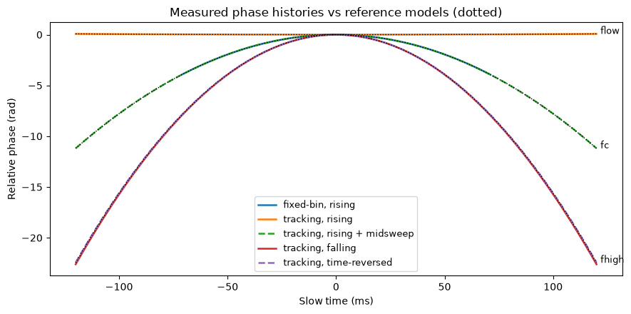
Reading the table: the tracking readout of a rising sweep is flow-referenced (RMS 0.000), using fcenter there would be a 5 rad RMS error over even this small aperture. The mid-sweep factor makes fcenter exact for rising and falling sweeps, which is what lets identical processing handle both sweep directions. Time reversal lands on the last-sample frequency f_last, not exactly fhigh. The fixed-bin readout is fcenter-referenced no matter what, because window leakage re-references it, a property of that readout, not of backprojection.

Backprojection with a DC-start sweep

Now with torchbp.ops.backprojection_polar_2d on real image formation. The stress test for point 2: flow = 0, B = 1.5 GHz. With first-sample-referenced data the correct carrier is fc = flow = 0, i.e. no phase compensation at all.

torchbp.util.generate_fmcw_data generates data referenced to the fc argument it is given (phase $2\pi(-f_c\tau - K\tau t + \tfrac12 K\tau^2)$). Real dechirped hardware data is referenced to the first ADC sample, so hardware-convention data is generated by passing the first-sample frequency as the carrier: flow for a rising sweep, fhigh (with bw < 0) for a falling one.

Three images of the same point target:

A: fc = 0, no re-referencing (consistent conventions),
B: fc = B/2 without re-referencing (mismatched: the image model assumes a mid-sweep reference the data do not have),
C: fc = B/2 with the mid-sweep factor (consistent again).

A and C should be identical and focused, B should defocus. The azimuth resolution of A is predicted from the physical spectral centroid (750 MHz, the signal energy is what it is), not from the fc parameter.

Implementing the mid-sweep factor with the backprojection kernel: at range bin index $s_x$ of the oversampled range profile the beat frequency is $f = s_x f_s/M$, so $e^{-j\pi f T} = e^{-j (\pi/\text{oversample})\, s_x}$: a pure linear phase across range bins. Multiplying the data with it would shift the data’s bin-domain spectrum away from DC and degrade the kernel’s linear interpolation. Instead it is folded into data_fmod, which the kernel removes exactly at the interpolated (fractional) bin position, equivalent, and interpolation accuracy is preserved. In this processing chain the falling-sweep branch conjugates the data, which flips the sign of the beat axis, hence the sign(bw) factor; with a signed beat-frequency axis the factor is always $e^{-j\pi f T}$.

[6]:

def range_compress(raw, bw, fs, tsweep, oversample, midsweep):
    '''Window + oversampled range FFT + spectrum centering, torchbp
    conventions. Optionally re-references the phase to mid sweep.'''
    nsamples = raw.shape[-1]
    M = nsamples * oversample
    w = torch.tensor(hamming(nsamples)[None, :], dtype=torch.float32)
    data_fmod = -np.pi * (1 - (oversample - 1) / oversample)
    if bw > 0:  # with a rising sweep the IF frequencies are negative
        data = torch.fft.ifft(raw * w, dim=-1, n=M)
    else:
        data = torch.fft.ifft(raw.conj() * w, dim=-1, n=M).conj()
        data_fmod = -data_fmod
    data = data * torch.exp(1j * data_fmod * torch.arange(M))[None, :]
    if midsweep:
        # exp(-1j*pi*f*tsweep) over the beat axis is a pure linear phase of
        # sign(bw)*pi/oversample rad/bin: fold it into data_fmod, which the
        # kernel removes exactly at the interpolated bin position.
        data_fmod = data_fmod + np.sign(bw) * np.pi / oversample
    return data, data_fmod

def peak_and_widths(img, grid):
    '''Peak value, peak (r, theta) and -3 dB widths of a polar image.'''
    a = torch.abs(img)
    ir, it = np.unravel_index(torch.argmax(a).item(), a.shape)
    r_ax = np.linspace(*grid["r"], grid["nr"], endpoint=False)
    t_ax = np.linspace(*grid["theta"], grid["ntheta"], endpoint=False)
    def w3db(cut, dx):
        aa = cut / cut.max()
        i0, lev = int(np.argmax(aa)), 10 ** (-3 / 20)
        def cross(d):
            i = i0
            while 0 < i < len(aa) - 1 and aa[i + d] > lev:
                i += d
            return i + d * (aa[i] - lev) / (aa[i] - aa[i + d])
        return (cross(1) - cross(-1)) * dx
    return (a[ir, it].item(), r_ax[ir], t_ax[it],
            w3db(a[:, it].numpy(), r_ax[1] - r_ax[0]),
            w3db(a[ir, :].numpy(), t_ax[1] - t_ax[0]))

[7]:

flow3 = 0.0 # hypothetical DC-start sweep
bw3 = 1.5e9
tsweep3 = 100e-6
fs3 = 12.8e6
oversample = 2
fcenter3 = flow3 + bw3 / 2
nsweeps = 256

pos = torch.zeros([nsweeps, 3], dtype=torch.float32)
pos[:, 1] = torch.linspace(-nsweeps / 2, nsweeps / 2, nsweeps) * 0.1
L = float(pos[-1, 1] - pos[0, 1])
target_pos = torch.tensor([[100.0, 0, 0]], dtype=torch.float32)
target_rcs = torch.tensor([[1.0]], dtype=torch.float32)

grid = {"r": (95.0, 105.0), "theta": (-0.03, 0.03), "nr": 256, "ntheta": 256}
r_res3 = c0 / (2 * bw3 * oversample)

# hardware convention: reference = first ADC sample -> generate with flow
raw = torchbp.util.generate_fmcw_data(target_pos, target_rcs, pos,
                                      flow3, bw3, tsweep3, fs3)

imgs = {}
for name, fc_bp, ms in [("A: fc = 0 (flow), no midsweep", 0.0, False),
                        ("B: fc = B/2, no midsweep", fcenter3, False),
                        ("C: fc = B/2, midsweep", fcenter3, True)]:
    data, data_fmod = range_compress(raw, bw3, fs3, tsweep3, oversample, ms)
    imgs[name] = torchbp.ops.backprojection_polar_2d(
        data, grid, fc_bp, r_res3, pos, data_fmod=data_fmod).squeeze()

names = list(imgs)
pkA = peak_and_widths(imgs[names[0]], grid)
for name, img in imgs.items():
    pk, r, th, rw, tw = peak_and_widths(img, grid)
    print(f"{name:30s} peak {20*np.log10(pk/pkA[0]):+6.2f} dB, "
          f"r = {r:.2f} m, theta = {th:+.4f}")
    print(f"   -3 dB widths: range {rw:.3f} m, azimuth {tw*r:.3f} m")

lam_c = c0 / fcenter3     # PHYSICAL spectral centroid, not the fc parameter
print(f"\nazimuth -3 dB width predicted from physical centroid "
      f"({fcenter3/1e6:.0f} MHz): {0.886 * lam_c * 100.0 / (2 * L):.3f} m")
print(f"range -3 dB width predicted (Hamming window): "
      f"{1.3 * c0 / (2 * bw3):.3f} m")
dmag = (imgs[names[0]].abs() - imgs[names[2]].abs()).abs().max().item()
print(f"max ||A| - |C|| / peak = {dmag/pkA[0]:.1e}  (A and C identical)")

A: fc = 0 (flow), no midsweep  peak  +0.00 dB, r = 100.08 m, theta = +0.0000
   -3 dB widths: range 0.133 m, azimuth 0.667 m
B: fc = B/2, no midsweep       peak -14.88 dB, r = 100.08 m, theta = +0.0073
   -3 dB widths: range 0.135 m, azimuth 3.827 m
C: fc = B/2, midsweep          peak  -0.00 dB, r = 100.08 m, theta = +0.0000
   -3 dB widths: range 0.133 m, azimuth 0.667 m

azimuth -3 dB width predicted from physical centroid (750 MHz): 0.692 m
range -3 dB width predicted (Hamming window): 0.130 m
max ||A| - |C|| / peak = 2.5e-03  (A and C identical)

[8]:

with plt.rc_context({"axes.grid": False}):
    fig, axs = plt.subplots(1, 3, figsize=(12, 3.6), sharey=True)
    extent = [*grid["theta"], *grid["r"]]
    for ax, name in zip(axs, names):
        db = 20 * torch.log10(imgs[name].abs() / pkA[0] + 1e-12)
        im = ax.imshow(db.numpy(), origin="lower", vmin=-20, vmax=0,
                       extent=extent, aspect="auto")
        ax.set_title(name, fontsize=10)
        ax.set_xlabel("Angle (sin radians)")
    axs[0].set_ylabel("Range (m)")
    fig.colorbar(im, ax=axs, shrink=0.9, label="dB rel. image A peak")

plt.figure(figsize=(8, 3.2))
t_ax = np.linspace(*grid["theta"], grid["ntheta"], endpoint=False)
for name, ls in zip(names, ["-", "-", "--"]):
    img = imgs[name]
    ir = np.unravel_index(img.abs().argmax().item(), img.shape)[0]
    cut = img.abs()[ir, :].numpy() / pkA[0]
    plt.plot(t_ax * 100.0, 20 * np.log10(cut + 1e-12),
             lw=1.8, ls=ls, label=name)
plt.ylim(-45, 2)
plt.xlabel("Cross-range at 100 m (m)")
plt.ylabel("dB rel. image A peak")
plt.title("Azimuth cuts through the point target (DC-start sweep)")
plt.legend(fontsize=9)
plt.tight_layout()

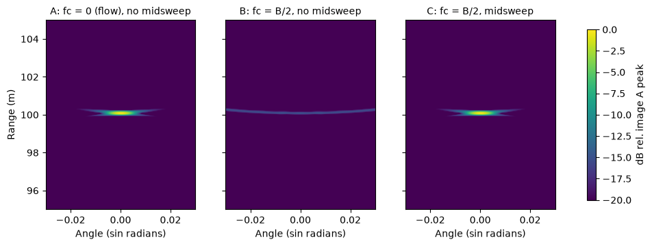
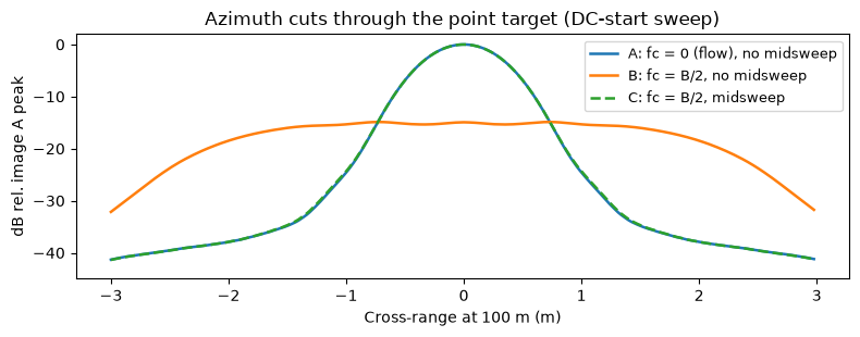
Image A focuses with fc = 0, the phase compensation is unity and the azimuth resolution still matches the prediction from the physical 750 MHz spectral centroid, because focusing information lives in the data. Image B, the mismatched convention, is badly defocused and shifted. Image C is identical to A in magnitude: fc = B/2 becomes correct once the data are actually re-referenced to mid sweep.

Note that A and C are only identical in magnitude: a complex SAR image formed with carrier fc carries an fc-dependent spatial phase ramp (this is why e.g. polar_to_cart and interferometric processing need the same fc the image was formed with).

One processing chain for rising and falling sweeps

The practical payoff of mid-sweep re-referencing: with fc = fcenter the same processing works for both sweep directions. A realistic 6 GHz / 200 MHz pair, without re-referencing the rising sweep would need fc = flow and the falling sweep fc = fhigh.

[9]:

fc_rf = 6e9
bw4 = 200e6
fs4 = 2e6
tsweep4 = 100e-6
pos4 = torch.zeros([nsweeps, 3], dtype=torch.float32)
pos4[:, 1] = torch.linspace(-nsweeps / 2, nsweeps / 2, nsweeps) * 0.25 * c0 / fc_rf
grid4 = {"r": (95.0, 105.0), "theta": (-0.03, 0.03), "nr": 256, "ntheta": 256}
r_res4 = c0 / (2 * bw4 * oversample)

# hardware convention: carrier = frequency at the first ADC sample
raw_rise = torchbp.util.generate_fmcw_data(
    target_pos, target_rcs, pos4, fc_rf - bw4 / 2, bw4, tsweep4, fs4)
raw_fall = torchbp.util.generate_fmcw_data(
    target_pos, target_rcs, pos4, fc_rf + bw4 / 2, -bw4, tsweep4, fs4)

res = {}
for name, raw4, bws in [("rising", raw_rise, bw4), ("falling", raw_fall, -bw4)]:
    data, data_fmod = range_compress(raw4, bws, fs4, tsweep4, oversample, True)
    res[name] = torchbp.ops.backprojection_polar_2d(
        data, grid4, fc_rf, r_res4, pos4, data_fmod=data_fmod).squeeze()
    pk, r, th, rw, tw = peak_and_widths(res[name], grid4)
    print(f"{name:8s} sweep, fc = fcenter + midsweep: "
          f"r = {r:.2f} m, theta = {th:+.4f}")
    print(f"   widths: range {rw:.3f} m, azimuth {tw*r:.3f} m")

d = (res["rising"].abs() - res["falling"].abs()).abs().max().item()
print(f"\nmax ||rising| - |falling|| / peak = "
      f"{d / res['rising'].abs().max().item():.1e}")
pr = res["rising"].flatten()[res["rising"].abs().argmax()].item()
pf = res["falling"].flatten()[res["falling"].abs().argmax()].item()
print(f"peak phase: rising {np.angle(pr):+.3f} rad, "
      f"falling {np.angle(pf):+.3f} rad")
print("   (difference is 2x the residual video phase; opposite signs "
      "for opposite sweeps)")

rising   sweep, fc = fcenter + midsweep: r = 100.12 m, theta = +0.0000
   widths: range 0.970 m, azimuth 0.688 m
falling  sweep, fc = fcenter + midsweep: r = 100.12 m, theta = +0.0000
   widths: range 0.970 m, azimuth 0.688 m

max ||rising| - |falling|| / peak = 1.8e-04
peak phase: rising +0.848 rad, falling +1.542 rad
   (difference is 2x the residual video phase; opposite signs for opposite sweeps)

Pulse compression radar

A pulse compression radar transmits a coded pulse, receives the full bandwidth and range compresses by correlating with a replica of the pulse (equivalently FFT, multiply by the conjugated reference spectrum, IFFT). Typically the data entering range compression is at DC-centered baseband: quadrature demodulation with the LO at the band centre, so the pulse spectrum spans $\pm B/2$ around $\mathrm{DC}$.

The structural difference to dechirp processing is that for correlation delay changes range origin instead of affecting the phase. What sets the phase reference instead is carrier removal: demodulating an echo delayed by $\tau$ with $e^{-j2\pi f_d t}$ leaves the compressed peak with phase $-2\pi f_d \tau$, so backprojection needs fc $= f_d$, the net demodulation frequency, which is the band center for DC-centered data. There is also no residual video phase with matched filtering.

The same phase-history experiment as earlier, on a wide-fractional-bandwidth pulse radar (0.5–1.5 GHz chirp pulse), with the manipulations that changed the dechirp reference:

record window delayed: the target moves to a smaller lag (a range-origin shift), the peak phase is unchanged,
ADC samples time-reversed (with the reference reversed consistently): the correlation output is exactly the same, compare with FMCW where reversal moved the dechirp reference to $f_{last}$,
LO not at the band centre (here at the band edge, band $0..B$): the reference follows the LO, not the band.

[10]:

fc5, bw5, tp5 = 1.0e9, 1.0e9, 0.5e-6   # RF band 0.5-1.5 GHz, 0.5 us pulse
fs5 = 3e9
ntp5 = int(round(tp5 * fs5))
nrec5 = int(round(1.0e-6 * fs5))
M5 = 8192 # >= nrec5 + ntp5: linear correlation
fax5 = np.fft.fftfreq(M5, 1 / fs5)

v5, R05, L5 = 50.0, 50.0, 12.0
nslow5 = 128
eta5 = np.linspace(-L5 / (2 * v5), L5 / (2 * v5), nslow5)
tau5 = 2 * np.sqrt((v5 * eta5)**2 + R05**2) / c0

def pulse_env(tt, tp, bw):
    '''Complex envelope of the TX pulse: DC-centred chirp, -B/2 to +B/2.'''
    K = bw / tp
    return np.where((tt >= 0) & (tt < tp),
                    np.exp(2j * np.pi * (-bw / 2 * tt + 0.5 * K * tt**2)), 0)

def compressed_peak_phase(f_demod, t0=0.0, reverse=False):
    '''Demodulate the echoes at f_demod, range compress by correlation with
    the demodulated replica and evaluate the correlation spectrum at the
    exact target lag, which is what backprojection's interpolation does.'''
    t_win = t0 + np.arange(nrec5) / fs5
    t_ref = np.arange(ntp5) / fs5
    foff = fc5 - f_demod              # residual carrier after demodulation
    out = []
    for tau in tau5:
        s = (pulse_env(t_win - tau, tp5, bw5)
             * np.exp(2j * np.pi * foff * (t_win - tau))
             * np.exp(-2j * np.pi * f_demod * tau))
        ref = pulse_env(t_ref, tp5, bw5) * np.exp(2j * np.pi * foff * t_ref)
        lag = tau - t0
        if reverse:
            s, ref = s[::-1], ref[::-1]
            lag = (nrec5 - 1) / fs5 - (ntp5 - 1) / fs5 - (tau - t0)
        Y = np.fft.fft(s, M5) * np.conj(np.fft.fft(ref, M5))
        out.append(np.sum(Y * np.exp(2j * np.pi * fax5 * lag)) / M5)
    return np.unwrap(np.angle(np.array(out)))

cases5 = {
    "DC-centred baseband (LO = band centre)":      compressed_peak_phase(fc5),
    "record window delayed 200 ns":                compressed_peak_phase(fc5, t0=200e-9),
    "ADC samples time-reversed":                   compressed_peak_phase(fc5, reverse=True),
    "LO at band edge (band 0..B, not DC-centred)": compressed_peak_phase(fc5 - bw5 / 2),
}
refs5 = {"flow": fc5 - bw5 / 2, "fc": fc5, "fhigh": fc5 + bw5 / 2}

print("peak-phase-history RMS mismatch (rad) vs reference model "
      f"(fc vs flow span = {2*np.pi*(bw5/2)*(tau5.max()-tau5.min()):.1f} rad):")
print(f"{'case':46s}" + "".join(f"{r:>9s}" for r in refs5) + "   winner")
for name, meas in cases5.items():
    r = {}
    for rn, fr in refs5.items():
        d = meas - (-2 * np.pi * fr * tau5)
        d = d - d[nslow5 // 2]        # constants are unobservable
        r[rn] = np.sqrt(np.mean(d**2))
    row = "".join(f"{r[rn]:9.3f}" for rn in refs5)
    print(f"{name:46s}{row}   {min(r, key=r.get)}")

peak-phase-history RMS mismatch (rad) vs reference model (fc vs flow span = 7.5 rad):
case                                               flow       fc    fhigh   winner
DC-centred baseband (LO = band centre)            3.416    0.000    3.416   fc
record window delayed 200 ns                      3.416    0.000    3.416   fc
ADC samples time-reversed                         3.416    0.000    3.416   fc
LO at band edge (band 0..B, not DC-centred)       0.000    3.416    6.831   flow

The winner is the demodulation frequency in every row: the time-origin and sample-order manipulations are invisible to the correlation readout.

Backprojection of pulse-compressed data

Same radar, now with torchbp.ops.backprojection_polar_2d. The range bin spacing is r_res $= c/(2 f_s \cdot \text{oversample})$ (oversampling by zero-padding the DC-centred product spectrum), bin 0 is at zero range, and the compressed data is used directly: the peak phase $-4\pi f_d R/c$ already matches the torchbp convention, no conjugation needed. Four images of the same point target:

A: DC-centred data, fc = fcenter (consistent conventions),
B: same data, fc = flow (wrong bookkeeping, 500 MHz off),
C: ADC window delayed by 250 ns, fc = fcenter unchanged: the delay is a pure range-origin shift, corrected with d0 $= -c t_0/2$, and the image should match A exactly, including phase. A dechirp window shift would instead have changed the required fc by $K t_0$.
D: LO offset 50 MHz below the band centre. The compressed profile then rides a residual carrier $e^{j2\pi f_{off}(l - \tau)}$ across the lag bins $l$. Folding it into data_fmod keeps the kernel’s interpolation accurate and moves the $-2\pi f_{off}\tau$ part of the phase into the compensation, so the total reference is $-2\pi(f_d + f_{off})\tau$ and fc = fcenter again: the bookkeeping mirror image of mid-sweep re-referencing.

[11]:

fs5b = 1.2e9
ntp5b = int(round(tp5 * fs5b))
nrec5b = int(round(1.5e-6 * fs5b))
M5b = 4096
nkeep5 = 2048
r_res5 = c0 / (2 * fs5b * oversample)

pos5 = torch.zeros([nsweeps, 3], dtype=torch.float32)
pos5[:, 1] = torch.linspace(-nsweeps / 2, nsweeps / 2, nsweeps) * 0.1
L5b = float(pos5[-1, 1] - pos5[0, 1])
tau5b = 2 * np.sqrt(100.0**2 + pos5[:, 1].numpy()**2) / c0
grid5 = {"r": (95.0, 105.0), "theta": (-0.06, 0.06), "nr": 256, "ntheta": 256}

def make_pulse_data(t0=0.0, f_demod=fc5):
    '''Echoes demodulated at f_demod; the record starts t0 after TX.'''
    t_win = t0 + np.arange(nrec5b) / fs5b
    foff = fc5 - f_demod
    return (pulse_env(t_win[None, :] - tau5b[:, None], tp5, bw5)
            * np.exp(2j * np.pi * foff * (t_win[None, :] - tau5b[:, None]))
            * np.exp(-2j * np.pi * f_demod * tau5b)[:, None])

def range_compress_pc(s, foff=0.0):
    '''Correlation range compression with a Hamming band taper and
    oversampled (zero-padded product spectrum) output.'''
    t_ref = np.arange(ntp5b) / fs5b
    ref = pulse_env(t_ref, tp5, bw5) * np.exp(2j * np.pi * foff * t_ref)
    fax = np.fft.fftfreq(M5b, 1 / fs5b)
    W = ((0.54 + 0.46 * np.cos(2 * np.pi * (fax - foff) / bw5))
         * (np.abs(fax - foff) <= bw5 / 2))
    Y = (np.fft.fft(s, M5b, axis=-1)
         * np.conj(np.fft.fft(ref, M5b))[None, :] * W[None, :])
    Yp = np.zeros((s.shape[0], oversample * M5b), complex)
    Yp[:, :M5b // 2] = Y[:, :M5b // 2]
    Yp[:, -(M5b // 2):] = Y[:, M5b // 2:]
    y = np.fft.ifft(Yp, axis=-1) * oversample
    return torch.tensor(y[:, :nkeep5], dtype=torch.complex64)

t0C = 250e-9                              # delayed ADC window for image C
foffD = 50e6                              # LO 50 MHz below band centre for D
data_pc = range_compress_pc(make_pulse_data())
data_pcC = range_compress_pc(make_pulse_data(t0C))
data_pcD = range_compress_pc(make_pulse_data(f_demod=fc5 - foffD), foff=foffD)
fmodD = 2 * np.pi * foffD / (fs5b * oversample)  # residual carrier, rad/bin

imgs5 = {}
for name, dat, fc_bp, d0, fmod in [
        ("A: fc = fcenter", data_pc, fc5, 0.0, 0.0),
        ("B: fc = flow", data_pc, fc5 - bw5 / 2, 0.0, 0.0),
        ("C: window +250 ns, fc = fcenter", data_pcC, fc5, -c0 * t0C / 2, 0.0),
        ("D: LO offset -50 MHz, data_fmod", data_pcD, fc5, 0.0, fmodD)]:
    imgs5[name] = torchbp.ops.backprojection_polar_2d(
        dat, grid5, fc_bp, r_res5, pos5, d0=d0, data_fmod=fmod).squeeze()

names5 = list(imgs5)
pkA5 = peak_and_widths(imgs5[names5[0]], grid5)
for name, img in imgs5.items():
    pk, r, th, rw, tw = peak_and_widths(img, grid5)
    print(f"{name:32s} peak {20*np.log10(pk/pkA5[0]):+6.2f} dB, "
          f"r = {r:.2f} m, theta = {th:+.4f}")
    print(f"   -3 dB widths: range {rw:.3f} m, azimuth {tw*r:.3f} m")

lam5 = c0 / fc5
print(f"\nazimuth -3 dB width predicted from the 1 GHz band centre: "
      f"{0.886 * lam5 * 100.0 / (2 * L5b):.3f} m")
print(f"range -3 dB width predicted (Hamming band taper): "
      f"{1.3 * c0 / (2 * bw5):.3f} m")
dAC = (imgs5[names5[0]] - imgs5[names5[2]]).abs().max().item()
print(f"max |A - C| / peak = {dAC/pkA5[0]:.1e}")
print("   (complex diff: window delay moved range origin, not phase ref)")
dAD = (imgs5[names5[0]] - imgs5[names5[3]]).abs().max().item()
print(f"max |A - D| / peak = {dAD/pkA5[0]:.1e}")
print("   (small linear-interpolation residual from carrier-riding bins)")

A: fc = fcenter                  peak  +0.00 dB, r = 100.00 m, theta = +0.0000
   -3 dB widths: range 0.198 m, azimuth 0.512 m
B: fc = flow                     peak -12.98 dB, r = 100.00 m, theta = +0.0098
   -3 dB widths: range 0.204 m, azimuth 6.053 m
C: window +250 ns, fc = fcenter  peak  +0.00 dB, r = 100.00 m, theta = +0.0000
   -3 dB widths: range 0.198 m, azimuth 0.512 m
D: LO offset -50 MHz, data_fmod  peak  -0.01 dB, r = 100.00 m, theta = +0.0000
   -3 dB widths: range 0.198 m, azimuth 0.513 m

azimuth -3 dB width predicted from the 1 GHz band centre: 0.519 m
range -3 dB width predicted (Hamming band taper): 0.195 m
max |A - C| / peak = 4.7e-11
   (complex diff: window delay moved range origin, not phase ref)
max |A - D| / peak = 7.3e-03
   (small linear-interpolation residual from carrier-riding bins)

[12]:

with plt.rc_context({"axes.grid": False}):
    fig, axs = plt.subplots(1, 4, figsize=(13, 3.2), sharey=True)
    extent = [*grid5["theta"], *grid5["r"]]
    for ax, name in zip(axs, names5):
        db = 20 * torch.log10(imgs5[name].abs() / pkA5[0] + 1e-12)
        im = ax.imshow(db.numpy(), origin="lower", vmin=-20, vmax=0,
                       extent=extent, aspect="auto")
        ax.set_title(name, fontsize=9)
        ax.set_xlabel("Angle (sin radians)")
    axs[0].set_ylabel("Range (m)")
    fig.colorbar(im, ax=axs, shrink=0.9, label="dB rel. image A peak")

plt.figure(figsize=(8, 3.2))
t_ax = np.linspace(*grid5["theta"], grid5["ntheta"], endpoint=False)
for name, ls in zip(names5, ["-", "-", "--", ":"]):
    img = imgs5[name]
    ir = np.unravel_index(img.abs().argmax().item(), img.shape)[0]
    cut = img.abs()[ir, :].numpy() / pkA5[0]
    plt.plot(t_ax * 100.0, 20 * np.log10(cut + 1e-12),
             lw=1.8, ls=ls, label=name)
plt.ylim(-45, 2)
plt.xlabel("Cross-range at 100 m (m)")
plt.ylabel("dB rel. image A peak")
plt.title("Azimuth cuts through the point target (pulse compression)")
plt.legend(fontsize=9)
plt.tight_layout()

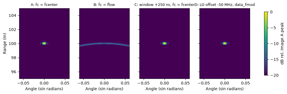
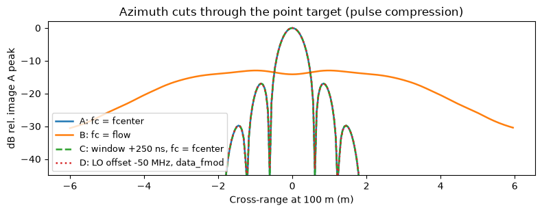
Image A focuses with the textbook fc = fcenter and matches the predicted widths. Image B shows that fc with 500 MHz error defocuses azimuth. C matches A to numerical precision in complex value, so the record window placement affects only the range origin, and D shows the offset-LO case restored to fc = fcenter by data_fmod.

Summary of the two waveform families: dechirp readouts inherit their phase reference from time-origin conventions (a single FFT maps delay to frequency, so linear-phase and origin conventions imprint on the phase vs range) and the required fc is therefore implementation-sensitive: flow, fcenter, fhigh or none of them, depending on window placement, sample order and re-referencing factors. Matched-filter readouts inherit the reference from the demodulation chain alone: fc equals the net frequency removed from the echo and is insensitive to windowing, trigger timing and sample order. With the usual DC-centered baseband convention that is fcenter.

[ ]: